---
title: "What the Equations Actually Say"
number-sections: true
---
::: {.callout-note icon=false}
## Learning Objectives
- Read each term in the Navier-Stokes equations and understand its physical meaning
- Understand the Hagen-Poiseuille solution for pipe flow
- Understand the Reynolds number as a dimensionless ratio of inertia to viscosity
- Visualize velocity profiles and the laminar-to-turbulent transition
:::
## Reading the Equations
The Navier-Stokes equations for an incompressible Newtonian fluid are:
$$\nabla \cdot \mathbf{u} = 0$$ {#eq-cont}
$$\rho \left( \frac{\partial \mathbf{u}}{\partial t} + \mathbf{u} \cdot \nabla \mathbf{u} \right) = -\nabla p + \mu \nabla^2 \mathbf{u} + \rho \mathbf{g}$$ {#eq-mom}
Two equations, one for mass and one for momentum. Four unknowns: three components of velocity $\mathbf{u} = (u, v, w)$ and pressure $p$.
@eq-cont says that the velocity field has no divergence --- fluid neither accumulates nor disappears. Any flow pattern consistent with this equation conserves mass at every point.
@eq-mom is the interesting one. Read it term by term:
**Left side:** $\rho \left( \partial_t \mathbf{u} + \mathbf{u} \cdot \nabla \mathbf{u} \right)$ is the inertial term --- mass per unit volume times acceleration. The $\partial_t \mathbf{u}$ piece is the local acceleration, the change in velocity at a fixed point as time passes. The $\mathbf{u} \cdot \nabla \mathbf{u}$ piece is the convective acceleration, the change in velocity that occurs because the fluid is moving through space where the velocity field is not uniform. This nonlinear term --- velocity times the gradient of velocity --- is where all the difficulty lives.
**$-\nabla p$:** Pressure gradient, pointing from high pressure to low. Fluids move downhill in pressure.
**$\mu \nabla^2 \mathbf{u}$:** The viscous term. The Laplacian $\nabla^2 \mathbf{u}$ measures how the velocity at a point differs from the average velocity of its surroundings --- a kind of smoothing operator. Multiply by $\mu$ and you have a force that drives the velocity toward uniformity. This is friction. This is the term that Navier and Stokes added to Euler.
**$\rho \mathbf{g}$:** Body force --- usually gravity.
The equation is Newton's second law for a fluid parcel, written per unit volume. It is not exotic or mysterious. What makes it hard is the $\mathbf{u} \cdot \nabla \mathbf{u}$ term, which makes the equations nonlinear and couples the three velocity components together.
## Pipe Flow
The simplest non-trivial solution of the Navier-Stokes equations is the one Navier himself could have computed: steady, fully developed flow through a circular pipe. Impose constant pressure gradient along the pipe, assume the flow is steady and purely axial, and the nonlinear term vanishes. What remains is a balance between pressure driving the flow and viscosity resisting it.
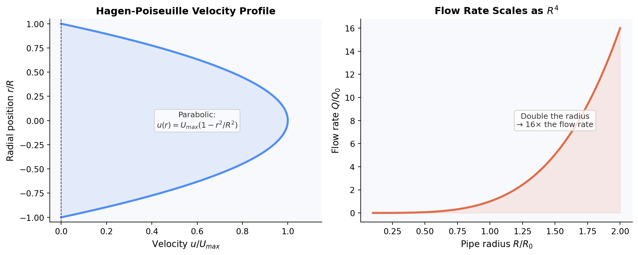
The solution is a parabola. The velocity is maximum at the center of the pipe and zero at the wall, varying as:
$$u(r) = \frac{\Delta p}{4 \mu L} (R^2 - r^2)$$ {#eq-poiseuille}
where $r$ is the distance from the centerline, $R$ is the pipe radius, $L$ is the pipe length, and $\Delta p$ is the pressure drop. This is the Hagen-Poiseuille profile.
```{python}
import numpy as np
import matplotlib.pyplot as plt
import matplotlib.gridspec as gridspec

fig, axes = plt.subplots(1, 2, figsize=(11, 4.5))

# Left: velocity profile across pipe cross-section
r = np.linspace(-1, 1, 400)
# Normalized: u(r) = 1 - r^2 (so U_max = 1 at r=0)
u = 1 - r**2

ax = axes[0]
ax.plot(u, r, color='#4f8ef7', linewidth=2.5)
ax.axvline(0, color='#2a2d3a', linewidth=0.8, linestyle='--')
ax.fill_betweenx(r, 0, u, alpha=0.12, color='#4f8ef7')
ax.set_xlabel('Velocity $u/U_{max}$', fontsize=11)
ax.set_ylabel('Radial position $r/R$', fontsize=11)
ax.set_title('Hagen-Poiseuille Velocity Profile', fontsize=12, fontweight='bold')
ax.set_xlim(-0.05, 1.15)
ax.set_ylim(-1.05, 1.05)
ax.spines['top'].set_visible(False)
ax.spines['right'].set_visible(False)
ax.set_facecolor('#f8f9fc')
ax.annotate('Parabolic:\n$u(r) = U_{max}(1 - r^2/R^2)$',
            xy=(0.6, 0.0), fontsize=9.5, color='#333',
            ha='center', va='center',
            bbox=dict(boxstyle='round,pad=0.3', fc='white', ec='#ccc', alpha=0.8))

# Right: flow rate vs radius (Q ~ R^4)
R_vals = np.linspace(0.1, 2.0, 200)
# Q = pi * delta_p * R^4 / (8 * mu * L) — normalized to Q=1 at R=1
Q = R_vals**4

ax2 = axes[1]
ax2.plot(R_vals, Q, color='#e06c4a', linewidth=2.5)
ax2.fill_between(R_vals, 0, Q, alpha=0.12, color='#e06c4a')
ax2.set_xlabel('Pipe radius $R/R_0$', fontsize=11)
ax2.set_ylabel('Flow rate $Q/Q_0$', fontsize=11)
ax2.set_title('Flow Rate Scales as $R^4$', fontsize=12, fontweight='bold')
ax2.spines['top'].set_visible(False)
ax2.spines['right'].set_visible(False)
ax2.set_facecolor('#f8f9fc')
ax2.annotate('Double the radius\n→ 16× the flow rate',
            xy=(1.5, 8), fontsize=9.5, color='#333',
            ha='center', va='center',
            bbox=dict(boxstyle='round,pad=0.3', fc='white', ec='#ccc', alpha=0.8))

plt.tight_layout()
plt.savefig('docs/pipe-flow.png', dpi=150, bbox_inches='tight')
plt.show()
```
The $R^4$ dependence in the Hagen-Poiseuille formula is striking. The volume flow rate through a pipe scales as the fourth power of the radius. Double the pipe diameter and you get sixteen times the flow rate at the same pressure. This relationship --- derived from @eq-mom in a few lines --- explains why arteries harden with age and why pipes sized correctly for a city water system must be sized correctly and cannot be easily undersized and compensated with increased pressure.
## The Reynolds Number
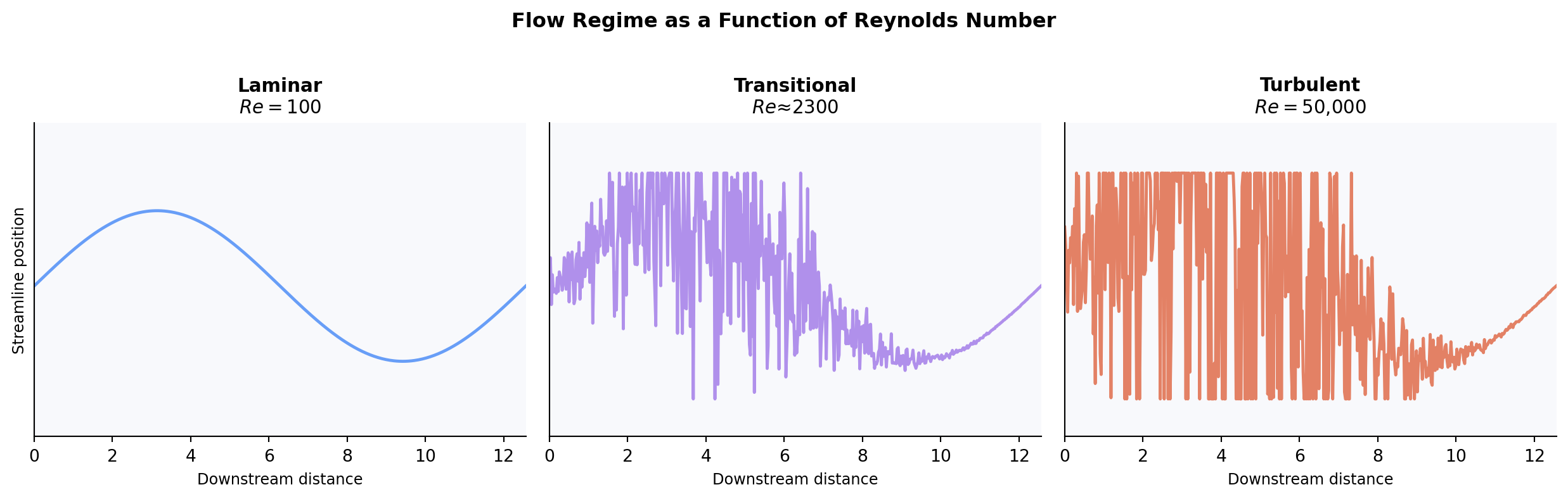
The Navier-Stokes equations contain two competing physical mechanisms: inertia (the $\mathbf{u} \cdot \nabla \mathbf{u}$ term) and viscosity (the $\mu \nabla^2 \mathbf{u}$ term). The ratio of their characteristic magnitudes defines the most important dimensionless parameter in fluid mechanics.
Scale the inertial term: $\rho |\mathbf{u} \cdot \nabla \mathbf{u}| \sim \rho U^2 / L$, where $U$ is a characteristic velocity and $L$ is a characteristic length.
Scale the viscous term: $\mu |\nabla^2 \mathbf{u}| \sim \mu U / L^2$.
Their ratio:
$$Re = \frac{\rho U L}{\mu} = \frac{U L}{\nu}$$ {#eq-reynolds}
where $\nu = \mu/\rho$ is the kinematic viscosity. This is the Reynolds number, named after Osborne Reynolds, who used it in 1883 to characterize the transition from smooth laminar flow to chaotic turbulent flow.
Low Reynolds number: viscosity dominates. The fluid behaves smoothly and predictably. Think of honey flowing out of a jar, or a bacterium swimming through water.
High Reynolds number: inertia dominates. The nonlinear term in @eq-mom becomes large relative to the viscous term, smooth solutions become unstable, and the flow transitions to turbulence.
```{python}
import numpy as np
import matplotlib.pyplot as plt

fig, axes = plt.subplots(1, 3, figsize=(13, 4))

x = np.linspace(0, 4 * np.pi, 500)
np.random.seed(42)

cases = [
    {'Re': 100,   'noise': 0.0,  'title': 'Laminar\n$Re = 100$',   'color': '#4f8ef7'},
    {'Re': 2300,  'noise': 0.15, 'title': 'Transitional\n$Re ≈ 2300$', 'color': '#a47ee8'},
    {'Re': 50000, 'noise': 0.45, 'title': 'Turbulent\n$Re = 50{,}000$', 'color': '#e06c4a'},
]

for ax, case in zip(axes, cases):
    y_base = np.sin(x * 0.5) * 0.3 + 0.5
    noise = np.random.normal(0, case['noise'], len(x))
    y = y_base + noise * np.exp(-0.1 * (x - np.pi)**2 + 0.2 * x)
    y = np.clip(y, 0.05, 0.95)

    ax.plot(x, y, color=case['color'], linewidth=1.8, alpha=0.85)
    ax.set_xlim(0, 4 * np.pi)
    ax.set_ylim(-0.1, 1.15)
    ax.set_title(case['title'], fontsize=11, fontweight='bold')
    ax.set_xlabel('Downstream distance', fontsize=9)
    if ax == axes[0]:
        ax.set_ylabel('Streamline position', fontsize=9)
    ax.set_yticks([])
    ax.spines['top'].set_visible(False)
    ax.spines['right'].set_visible(False)
    ax.set_facecolor('#f8f9fc')

plt.suptitle('Flow Regime as a Function of Reynolds Number', fontsize=12, fontweight='bold', y=1.02)
plt.tight_layout()
plt.savefig('docs/reynolds-regimes.png', dpi=150, bbox_inches='tight')
plt.show()
```
The Reynolds number is one of the most useful single numbers in engineering. A pipe flow with $Re < 2300$ is reliably laminar; above $Re \approx 4000$ it is reliably turbulent; in between, it may be either depending on disturbances. A wing with $Re \approx 10^6$ carries turbulent boundary layers on most of its surface. A bacterium swimming at $Re \approx 10^{-4}$ lives in a world where viscosity is overwhelming and inertia is negligible.
Same equations, same parameters, wildly different behaviors depending on their ratio.
## Summary
The Navier-Stokes momentum equation is Newton's second law for a fluid parcel, with terms representing local acceleration, convective acceleration, pressure, viscous diffusion, and body forces. The nonlinear convective term is the source of mathematical difficulty. The Hagen-Poiseuille solution for pipe flow --- a parabolic velocity profile with flow rate proportional to $R^4$ --- is the simplest exact solution and follows directly from the equations. The Reynolds number, the ratio of inertial to viscous forces, determines whether a flow is laminar, transitional, or turbulent. High Reynolds number is where the equations become practically unsolvable in closed form.
## Further Reading
- White, F.M. *Fluid Mechanics*, 8th ed. McGraw-Hill, 2015. Chapter 6 covers pipe flow; Chapter 1 covers viscosity.
- Reynolds, O. "An experimental investigation of the circumstances which determine whether the motion of water shall be direct or sinuous." *Philosophical Transactions of the Royal Society*, 174 (1883): 935–982. The original description of the transition to turbulence.
- Batchelor, G.K. *An Introduction to Fluid Dynamics*. Cambridge University Press, 1967. The standard graduate text; Chapter 4 covers viscous flow.