6 The Bent Beam
6.1 The Beam Reconsidered
Galileo’s cantilever problem, which we visited in the first chapter, sat unresolved for most of the seventeenth century. The missing ingredient was Hooke’s Law. With it — with the knowledge that stress is proportional to strain, and that strain in a bent beam varies linearly with distance from the neutral axis — the problem becomes tractable. Without it, the stress distribution across the cross-section is a guess, and Galileo’s guess was wrong.
By the late eighteenth century, the tools were in place. Young’s Modulus existed as a material property. The geometry of bending had been studied by Jacob Bernoulli and, more rigorously, by Euler. What emerged from their combined effort is now called Euler-Bernoulli beam theory, and it remains the foundation of structural design for beams, girders, joists, and virtually every other horizontal load-carrying member in common use.
6.2 How a Beam Bends
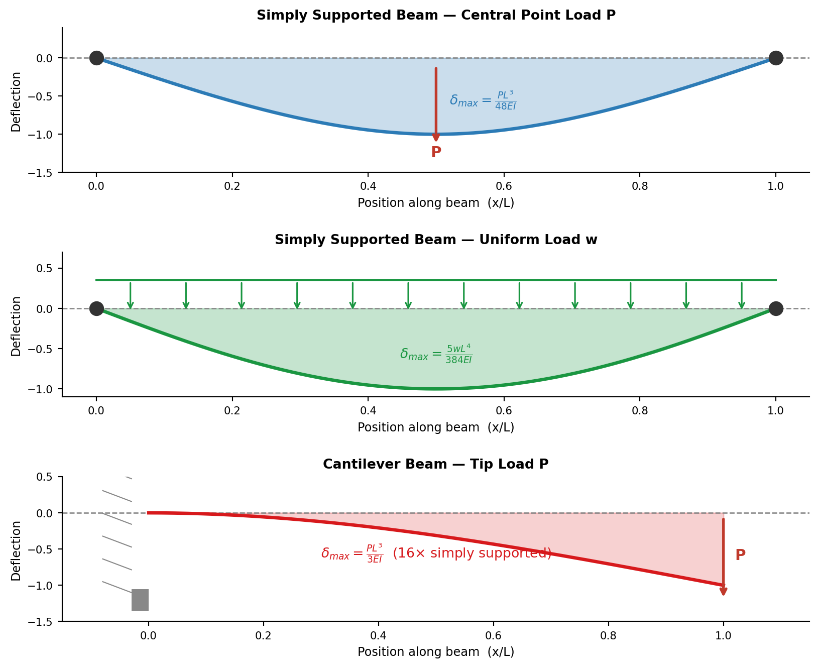
Imagine a simply supported beam — horizontal, resting on supports at both ends, carrying a load somewhere in the middle. Under the load, the beam sags. The top surface is compressed; the material there has gotten shorter. The bottom surface is stretched; the material there has gotten longer. Somewhere between top and bottom, the material has changed length by exactly zero — it is neither compressed nor stretched. This is the neutral axis.
Hooke’s Law requires that the stress at any point in the cross-section be proportional to the strain at that point, which is proportional to the distance from the neutral axis. The stress distribution is therefore linear: zero at the neutral axis, maximum at the outer fibers, tensile below and compressive above (for a downward load). This is precisely what Mariotte guessed and what Galileo missed. The mathematical proof that this is the only consistent distribution for a material obeying Hooke’s Law came later, but the physical intuition was correct.
The bending moment \(M\) at a cross-section — the net turning effect of all the external forces to one side of that section — must be balanced by the internal stress distribution. Working through the geometry and applying Hooke’s Law, one arrives at the fundamental relationship:
\[M = EI\kappa \tag{6.1}\]
In this equation, \(E\) is Young’s Modulus, \(I\) is the second moment of area of the cross-section about the neutral axis, and \(\kappa\) is the curvature of the beam at that point — how sharply the beam is bent. For small deflections, the curvature is approximately equal to the second derivative of the deflection \(y\) with respect to the axial position \(x\), giving the differential equation that governs beam deflection:
\[EI\frac{d^2y}{dx^2} = M(x) \tag{6.2}\]
This is the Euler-Bernoulli beam equation, and it contains Hooke’s Law in its DNA. The \(E\) is Young’s Modulus; the \(I\) is geometry; the product \(EI\) is called the flexural rigidity of the beam. Double the modulus and the beam deflects half as much. Double the second moment of area and the beam deflects half as much. The two effects are interchangeable, which is a significant design insight.
6.3 The Second Moment of Area
The second moment of area, \(I\), is worth examining carefully, because it explains one of the most consequential design decisions in structural engineering: the shape of the cross-section.
For a rectangular cross-section of width \(b\) and height \(h\), the second moment of area about the horizontal neutral axis is:
\[I = \frac{bh^3}{12} \tag{6.3}\]
The cubic dependence on height is striking. Double the height of a rectangular beam and you multiply its bending stiffness by eight — not two, not four, but eight. A beam twice as tall is eight times stiffer in bending. This is why tall beams carry bending loads more efficiently than wide, flat ones.
But there is a subtlety. The second moment of area rewards material that is far from the neutral axis. Material near the neutral axis contributes little to bending resistance — its stress and strain are both small. Material at the outer fibers contributes the most. A solid rectangular section carries material at all distances from the neutral axis, including the low-value region near the center. A hollow section, or an I-shaped section, removes material from near the center and concentrates it at the flanges, where it does the most good.
This is the engineering logic of the I-beam. By concentrating material in the flanges — far from the neutral axis — and using a thin web to connect them and carry shear, the I-beam achieves a high second moment of area with a relatively small cross-sectional area, meaning high bending stiffness with low material consumption. The I-beam is not an aesthetic preference or a manufacturing accident. It is the direct structural consequence of Hooke’s Law applied to bending.
6.4 Euler’s Column
Beams carry load in bending. Columns carry load in compression. The behavior of slender columns under compressive load is governed by a relationship that Euler derived in 1744 — the same Euler who co-developed beam bending theory — and it reveals one of the more unsettling truths in structural mechanics: a column can fail not by being crushed but by suddenly springing sideways.
This phenomenon is called buckling, and it illustrates something subtle about Hooke’s Law’s role in structural behavior. The material inside a column under compressive load is behaving exactly as Hooke’s Law predicts — stress proportional to strain, perfectly elastic, no permanent deformation. And yet the column fails. It fails not because the material yields, but because the straight configuration becomes geometrically unstable.
Euler showed that there is a critical load, \(P_{cr}\), at which a perfectly straight, perfectly uniform column will buckle:
\[P_{cr} = \frac{\pi^2 EI}{(KL)^2} \tag{6.4}\]
In this equation, \(E\) is Young’s Modulus, \(I\) is the second moment of area of the cross-section (the same one that governs bending), \(L\) is the length of the column, and \(K\) is an effective length factor that depends on how the column’s ends are constrained. A column pinned at both ends has \(K = 1\). A column fixed at both ends has \(K = 0.5\), meaning it behaves like a column of half the length and carries four times the buckling load.
The factor \((KL)^2\) in the denominator is telling. Buckling load decreases with the square of the effective length. Double the length and the critical load drops by a factor of four. This explains why slender columns fail at loads far below the material’s compressive strength: the geometry defeats the material.
The ratio \(KL/r\) — where \(r\) is the radius of gyration, \(r = \sqrt{I/A}\), a geometric property of the cross-section — is called the slenderness ratio. It is the single number that determines whether a column will buckle before it yields. High slenderness: buckling governs. Low slenderness: material crushing governs. The dividing line depends on the material’s modulus and yield stress. For structural steel, columns with slenderness ratios above about 100 are firmly in the buckling-governed regime.
6.5 Correcting Galileo
With the Euler-Bernoulli beam equation in hand, we can finally resolve the error that Galileo made in 1638.
Galileo placed all the tensile resistance at the bottom fiber of the cantilever’s cross-section, giving his formula for breaking load a fixed end moment equal to the force times the beam height. The correct analysis, using Hooke’s Law and the section modulus \(S = I/c\) (where \(c\) is the distance from the neutral axis to the outer fiber), gives a breaking condition of:
\[\sigma_{max} = \frac{Mc}{I} = \frac{M}{S} \tag{6.5}\]
For a rectangular cross-section of width \(b\) and height \(h\): \(I = bh^3/12\), \(c = h/2\), and \(S = bh^2/6\). Galileo’s formula, by contrast, effectively used a section modulus of \(bh^2/2\) — three times larger. He overestimated the strength by a factor of three. Mariotte’s correction, placing the neutral axis at the centroid, was qualitatively right but lacked the quantitative derivation. The full derivation required Hooke’s Law, the concept of Young’s Modulus, and the integration of stresses across the cross-section — tools that became available incrementally over the century following Galileo.
Galileo was not a sloppy thinker. He was solving a problem that required mathematical tools which did not exist in his lifetime. His error was, in a meaningful sense, not his fault. It was the fault of the missing law that a younger, querulous, brilliant man named Hooke would discover thirty years after Galileo’s death.