---
title: "Linear Algebra Foundations for Operations Research and Machine Learning"
subtitle: "Chapter 1 – Part I: Foundations"
author: "Troy Altus"
date: "2026-04-12"
number-sections: true
number-depth: 3
---
## Why Linear Algebra Matters in OR and ML {#sec-why-linalg}
Linear algebra is the mathematical scaffolding that connects optimization and machine
learning. It provides a compact, powerful language for expressing problems that would
otherwise require hundreds of individual equations.
In **Operations Research**, linear algebra underpins:
- Representing decision variables as vectors
- Encoding constraints as matrix inequalities ($Ax \leq b$)
- Solving systems of equations at the heart of the Simplex Method
- Sensitivity analysis and dual variable computation
In **Machine Learning**, it powers:
- Data representation — every dataset is a matrix of features
- Gradient computation and weight updates in neural networks
- Dimensionality reduction via PCA and SVD
- Distance and similarity metrics for clustering and nearest-neighbour methods
The table below maps key linear algebra concepts to their roles across both fields.
| Concept | Operations Research Role | Machine Learning Role |
|---|---|---|
| Vectors | Decision variables, constraint coefficients | Feature vectors, gradient vectors |
| Matrices | Constraint matrix $A$, cost matrix | Design matrix $X$, weight matrices |
| Linear systems | $Ax = b$ — solving LP at optimum | Normal equations for linear regression |
| Eigendecomposition | Sensitivity, covariance structure | PCA directions, stability analysis |
| SVD | Reduced-form models | Dimensionality reduction, recommender systems |
---
## Vectors {#sec-vectors}
### Intuition and Definition
A vector is an ordered list of numbers. Geometrically, it is an arrow with both
**direction** and **magnitude**. In OR and ML contexts, vectors are everywhere:
- A **production plan** for three products: $\mathbf{x} = [100, 150, 80]^T$
- A **customer's features**: $\mathbf{x} = [\text{age}, \text{income}, \text{tenure}]^T$
- A **gradient**: $\nabla f(\mathbf{w}) = [\partial f/\partial w_1, \ldots, \partial f/\partial w_n]^T$
Formally, a vector $\mathbf{v} \in \mathbb{R}^n$ is an element of $n$-dimensional real space:
$$\mathbf{v} = \begin{bmatrix} v_1 \\ v_2 \\ \vdots \\ v_n \end{bmatrix}$$
```{python}
#| label: vector-basics
import numpy as np
import matplotlib.pyplot as plt
import matplotlib.patches as mpatches

# Production plan vector
production = np.array([100, 150, 80])
print("Production vector:", production)
print("Shape:", production.shape)
print("Number of elements (dimensions):", production.size)
```
### Vector Operations
**Scalar multiplication** scales every component uniformly — increasing production by 20%:
$$\alpha \mathbf{v} = \alpha \begin{bmatrix} v_1 \\ v_2 \\ v_3 \end{bmatrix} = \begin{bmatrix} \alpha v_1 \\ \alpha v_2 \\ \alpha v_3 \end{bmatrix}$$
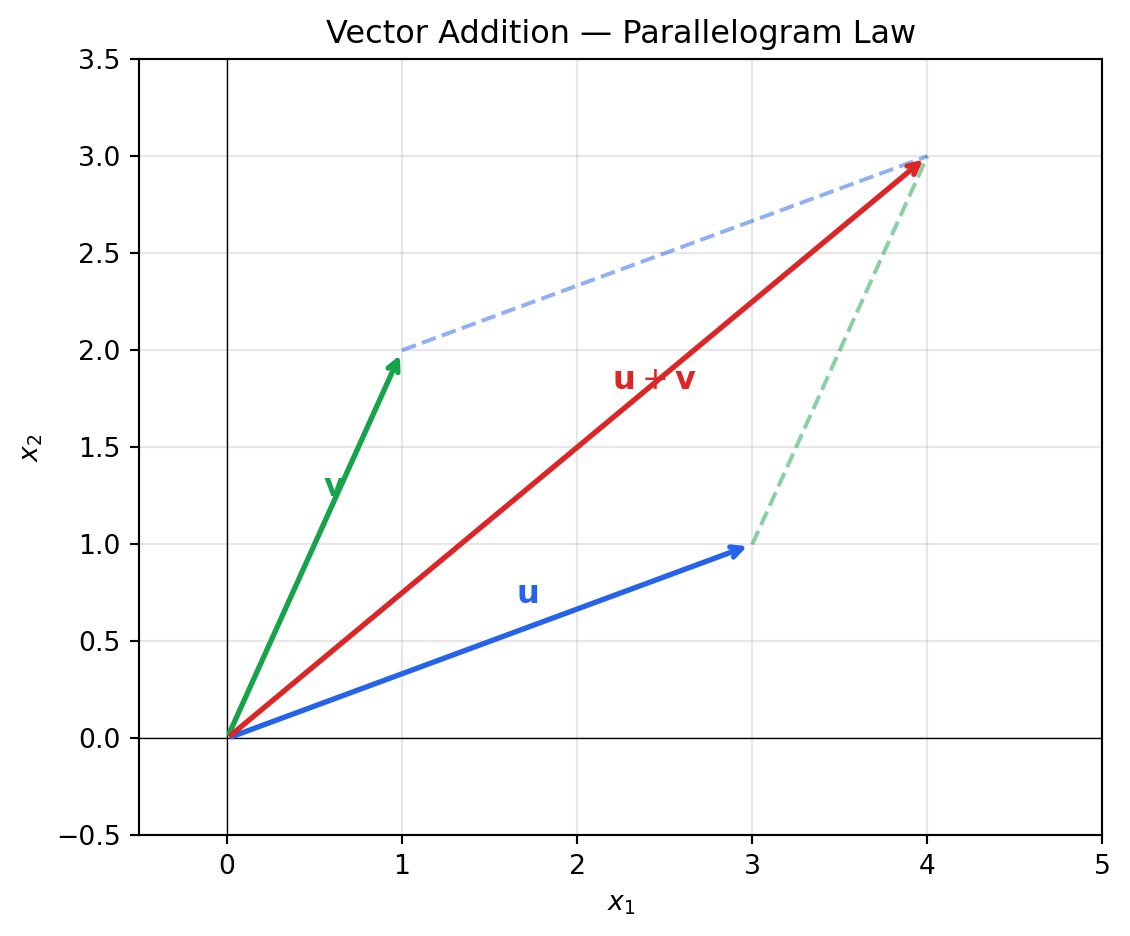
**Vector addition** combines two plans — adding an emergency order on top of a base plan:
$$\mathbf{u} + \mathbf{v} = \begin{bmatrix} u_1 + v_1 \\ u_2 + v_2 \\ u_3 + v_3 \end{bmatrix}$$
```{python}
#| label: vector-operations
base_plan   = np.array([100, 150, 80])
extra_order = np.array([10, 20, 5])

# Scalar multiplication: ramp up all production by 20%
scaled = 1.2 * base_plan
print("Scaled plan (×1.2):    ", scaled)

# Vector addition: add emergency order
total = base_plan + extra_order
print("Total with extra order:", total)

# Subtraction: compare two plans
delta = base_plan - extra_order
print("Net difference:        ", delta)
```
### The Dot Product
The dot product of two vectors $\mathbf{u}$ and $\mathbf{v}$ is:
$$\mathbf{u} \cdot \mathbf{v} = \sum_{i=1}^{n} u_i v_i = \|\mathbf{u}\| \|\mathbf{v}\| \cos\theta$$
where $\theta$ is the angle between the vectors. In OR, the dot product computes the
**total profit** from a production plan — multiplying quantities by unit profits:
$$\text{Profit} = \mathbf{c} \cdot \mathbf{x} = c_1 x_1 + c_2 x_2 + c_3 x_3$$
In ML, it measures **similarity** between a weight vector and a feature vector —
the core operation inside every linear layer of a neural network.
```{python}
#| label: dot-product
unit_profits = np.array([40, 30, 55])   # $/unit for products A, B, C
production   = np.array([100, 150, 80])

# Total profit via dot product
total_profit = np.dot(unit_profits, production)
print(f"Total profit: ${total_profit:,}")

# Verify manually
manual = sum(p * q for p, q in zip(unit_profits, production))
print(f"Manual check: ${manual:,}")

# Geometric interpretation: cos(theta) between two vectors
u = np.array([3.0, 4.0])
v = np.array([1.0, 2.0])

cos_theta = np.dot(u, v) / (np.linalg.norm(u) * np.linalg.norm(v))
theta_deg = np.degrees(np.arccos(cos_theta))
print(f"\nAngle between u={u} and v={v}: {theta_deg:.1f}°")
```
### Vector Norms and Distance
The **norm** of a vector measures its magnitude — the "length" of the arrow.
The most common is the **Euclidean norm** (L2 norm):
$$\|\mathbf{v}\|_2 = \sqrt{\sum_{i=1}^n v_i^2}$$
The **L1 norm** (Manhattan distance) sums absolute values:
$$\|\mathbf{v}\|_1 = \sum_{i=1}^n |v_i|$$
Norms appear throughout both fields:
- **OR**: constraint violation is measured by $\|Ax - b\|$
- **ML regression**: minimizing $\|y - X\beta\|_2^2$ gives least squares; L1 regularisation
(Lasso) uses $\|\beta\|_1$ to force sparsity
```{python}
#| label: vector-norms
v = np.array([3.0, 4.0])   # classic 3-4-5 triangle

l2 = np.linalg.norm(v)          # sqrt(9 + 16) = 5
l1 = np.linalg.norm(v, ord=1)   # 3 + 4 = 7

print(f"Vector: {v}")
print(f"L2 norm: {l2:.2f}  (Euclidean length)")
print(f"L1 norm: {l1:.2f}  (Manhattan distance)")

# Distance between two points in feature space
customer_a = np.array([35, 72000, 3])   # age, income, tenure
customer_b = np.array([42, 85000, 7])

euclidean_dist = np.linalg.norm(customer_a - customer_b)
print(f"\nEuclidean distance between customers: {euclidean_dist:.2f}")
```
### Visualising Vectors in 2D
```{python}
#| label: fig-vectors-2d
#| fig-cap: "Vector addition illustrated geometrically. The sum u + v reaches the same point whether you traverse u then v, or v then u (parallelogram law)."
fig, ax = plt.subplots(figsize=(6, 5))

u = np.array([3, 1])
v = np.array([1, 2])
w = u + v

origin = np.zeros(2)

for vec, color, label in [(u, "#2563eb", r"$\mathbf{u}$"),
                           (v, "#16a34a", r"$\mathbf{v}$"),
                           (w, "#dc2626", r"$\mathbf{u}+\mathbf{v}$")]:
    ax.annotate("", xy=vec, xytext=origin,
                arrowprops=dict(arrowstyle="->", color=color, lw=2))
    ax.text(vec[0] * 0.55, vec[1] * 0.55 + 0.15, label, color=color, fontsize=12)

# Parallelogram dashed lines
ax.plot([u[0], w[0]], [u[1], w[1]], "--", color="#16a34a", alpha=0.5)
ax.plot([v[0], w[0]], [v[1], w[1]], "--", color="#2563eb", alpha=0.5)

ax.set_xlim(-0.5, 5)
ax.set_ylim(-0.5, 3.5)
ax.axhline(0, color="black", linewidth=0.5)
ax.axvline(0, color="black", linewidth=0.5)
ax.grid(True, alpha=0.3)
ax.set_xlabel("$x_1$"); ax.set_ylabel("$x_2$")
ax.set_title("Vector Addition — Parallelogram Law")
plt.tight_layout()
plt.show()
```
---
## Matrices {#sec-matrices}
### Intuition and Definition
A matrix is a two-dimensional array of numbers. It generalises the idea of a vector
from a single list to a grid with rows and columns.
In OR, the **constraint matrix** $A \in \mathbb{R}^{m \times n}$ encodes all resource
requirements: row $i$ is resource $i$, column $j$ is product $j$, and entry $a_{ij}$
is how much of resource $i$ product $j$ consumes.
In ML, the **design matrix** $X \in \mathbb{R}^{N \times p}$ holds the dataset: row
$i$ is observation $i$, column $j$ is feature $j$.
$$A = \begin{bmatrix}
a_{11} & a_{12} & \cdots & a_{1n} \\
a_{21} & a_{22} & \cdots & a_{2n} \\
\vdots & & \ddots & \vdots \\
a_{m1} & a_{m2} & \cdots & a_{mn}
\end{bmatrix}$$
```{python}
#| label: matrix-basics
import numpy as np

# Constraint matrix for a 3-product, 2-resource LP
# Row 0 = machine hours, Row 1 = labour hours
# Col 0 = Product A, Col 1 = Product B, Col 2 = Product C
A = np.array([
    [4, 2, 3],   # machine hours per unit
    [2, 3, 1],   # labour hours per unit
])

b = np.array([160, 120])   # available hours

print("Constraint matrix A:")
print(A)
print(f"\nShape: {A.shape}  →  {A.shape[0]} constraints, {A.shape[1]} products")
print(f"Capacity vector b: {b}")
```
### Matrix Operations
**Matrix–vector multiplication** $A\mathbf{x}$ applies the transformation encoded in
$A$ to the vector $\mathbf{x}$. In LP, $A\mathbf{x}$ gives the total resource
consumption of a production plan:
$$A\mathbf{x} = \begin{bmatrix} \text{machine hours used} \\ \text{labour hours used} \end{bmatrix}$$
```{python}
#| label: matrix-vector-mult
A = np.array([[4, 2, 3],
              [2, 3, 1]])

x = np.array([20, 30, 10])   # production plan

resource_usage = A @ x
print(f"Production plan: {x}")
print(f"Resource usage:  {resource_usage}")
print(f"Capacity:        [160, 120]")
print(f"Feasible?        {all(resource_usage <= [160, 120])}")
```
**Matrix–matrix multiplication** $C = AB$ composes two linear transformations. Entry
$c_{ij} = \sum_k a_{ik} b_{kj}$ — the dot product of row $i$ of $A$ with column $j$ of $B$.
```{python}
#| label: matrix-multiply
A = np.array([[1, 2],
              [3, 4]])
B = np.array([[5, 6],
              [7, 8]])

C = A @ B
print("A @ B =")
print(C)

# Note: matrix multiplication is NOT commutative in general
print("\nB @ A =")
print(B @ A)
print(f"\nA@B == B@A?  {np.allclose(C, B @ A)}")
```
**Transpose** $A^T$ flips rows and columns. $(A^T)_{ij} = A_{ji}$.
```{python}
#| label: transpose
A = np.array([[1, 2, 3],
              [4, 5, 6]])

print("A:")
print(A)
print(f"Shape: {A.shape}")

print("\nA.T:")
print(A.T)
print(f"Shape: {A.T.shape}")
```
### Special Matrices
Several matrix structures appear repeatedly in OR and ML:
| Name | Definition | Significance |
|---|---|---|
| Identity $I$ | $I_{ij} = 1$ if $i=j$, else $0$ | $AI = IA = A$ |
| Diagonal | Non-zero only on main diagonal | Scaling transformation |
| Symmetric | $A = A^T$ | Covariance matrices, Hessians |
| Orthogonal | $A^T A = I$ | Rotation/reflection — preserves length |
| Positive Definite | $\mathbf{x}^T A \mathbf{x} > 0$ for all $\mathbf{x} \neq 0$ | Convex quadratic forms |
```{python}
#| label: special-matrices
n = 4

# Identity matrix
I = np.eye(n)
print("Identity (4×4):")
print(I)

# Diagonal matrix
D = np.diag([2.0, 3.0, 0.5, 1.0])
print("\nDiagonal matrix:")
print(D)

# Symmetric matrix (e.g., a covariance matrix)
data = np.random.default_rng(42).normal(size=(100, 3))
cov = np.cov(data.T)
print(f"\nCovariance matrix (3×3, symmetric: {np.allclose(cov, cov.T)}):")
print(np.round(cov, 3))
```
### The Matrix Inverse
For a square matrix $A$, the inverse $A^{-1}$ satisfies $A A^{-1} = A^{-1} A = I$.
It exists only when $A$ is **non-singular** (full rank, determinant $\neq 0$).
Inverses are important in theory but rarely computed directly in practice — solving
$Ax = b$ via `np.linalg.solve` is numerically more stable than $x = A^{-1}b$.
```{python}
#| label: matrix-inverse
A = np.array([[2.0, 1.0],
              [5.0, 3.0]])

A_inv = np.linalg.inv(A)
print("A:")
print(A)
print("\nA⁻¹:")
print(A_inv)
print("\nA @ A⁻¹ (should be I):")
print(np.round(A @ A_inv, 10))

# Determinant — zero means singular (not invertible)
print(f"\ndet(A) = {np.linalg.det(A):.4f}")
```
---
## Systems of Linear Equations {#sec-linear-systems}
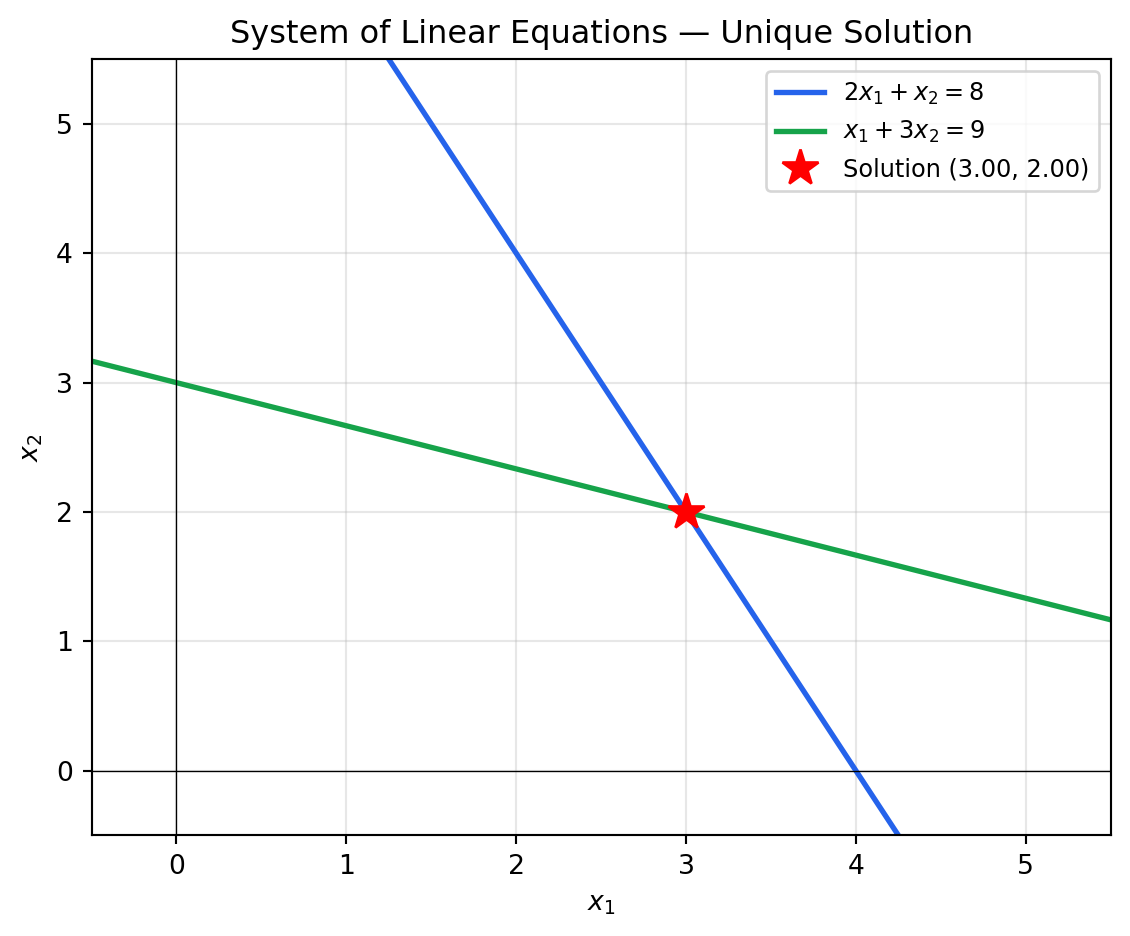
### Structure and Geometric Interpretation
A linear system $A\mathbf{x} = \mathbf{b}$ with $m$ equations and $n$ unknowns is
the computational core of linear programming. Every LP, when solved at an optimal
vertex, reduces to solving a square linear system of active constraints.
In 2D, each equation is a **line**; in 3D, a **plane**; in $n$ dimensions, a
**hyperplane**. The solution is the intersection of these hyperplanes.
```{python}
#| label: fig-linear-system
#| fig-cap: "Two linear equations intersect at a unique solution point. In LP, this corresponds to an optimal corner of the feasible region."
fig, ax = plt.subplots(figsize=(6, 5))

x = np.linspace(-1, 6, 300)

# System: 2x + y = 8  and  x + 3y = 9
line1 = 8 - 2 * x
line2 = (9 - x) / 3

ax.plot(x, line1, color="#2563eb", lw=2, label=r"$2x_1 + x_2 = 8$")
ax.plot(x, line2, color="#16a34a", lw=2, label=r"$x_1 + 3x_2 = 9$")

# Solve the system
A_sys = np.array([[2, 1], [1, 3]])
b_sys = np.array([8, 9])
sol = np.linalg.solve(A_sys, b_sys)

ax.plot(*sol, "r*", ms=14, zorder=5, label=f"Solution ({sol[0]:.2f}, {sol[1]:.2f})")
ax.axhline(0, color="black", lw=0.5)
ax.axvline(0, color="black", lw=0.5)
ax.set_xlim(-0.5, 5.5)
ax.set_ylim(-0.5, 5.5)
ax.grid(True, alpha=0.3)
ax.legend(fontsize=9)
ax.set_xlabel("$x_1$"); ax.set_ylabel("$x_2$")
ax.set_title("System of Linear Equations — Unique Solution")
plt.tight_layout()
plt.show()
```
### Solving Linear Systems in NumPy
```{python}
#| label: solve-system
# System of 3 equations, 3 unknowns
# Resource allocation at optimality in a 3-product LP
A = np.array([
    [2.0,  1.0,  1.0],
    [4.0,  3.0,  2.0],
    [1.0,  2.0,  3.0],
])
b = np.array([10.0, 22.0, 14.0])

# Solve Ax = b
x = np.linalg.solve(A, b)
print(f"Solution x = {x}")
print(f"Verification Ax = {A @ x}  (should equal b = {b})")
print(f"Residual ‖Ax − b‖₂ = {np.linalg.norm(A @ x - b):.2e}")
```
### Existence and Uniqueness
A system $A\mathbf{x} = \mathbf{b}$ has:
- **Unique solution** when $A$ is square and full rank ($\det A \neq 0$)
- **No solution** (inconsistent) when the equations are contradictory
- **Infinitely many solutions** when the system is underdetermined ($m < n$) or
$A$ is rank-deficient
In OR, the **rank** of the constraint matrix determines whether an LP has a unique
optimal solution, infinitely many optimal solutions, or is infeasible.
```{python}
#| label: rank-demo
A_full  = np.array([[1, 0], [0, 1]])   # rank 2 — unique solution
A_rank1 = np.array([[1, 2], [2, 4]])   # rank 1 — row 2 = 2×row 1, infinite solutions

print(f"rank(full matrix):        {np.linalg.matrix_rank(A_full)}")
print(f"rank(rank-deficient):     {np.linalg.matrix_rank(A_rank1)}")
print(f"det(full matrix):         {np.linalg.det(A_full):.2f}")
print(f"det(rank-deficient):      {np.linalg.det(A_rank1):.2f}")
```
---
## Eigenvalues and Eigenvectors {#sec-eigenvalues}
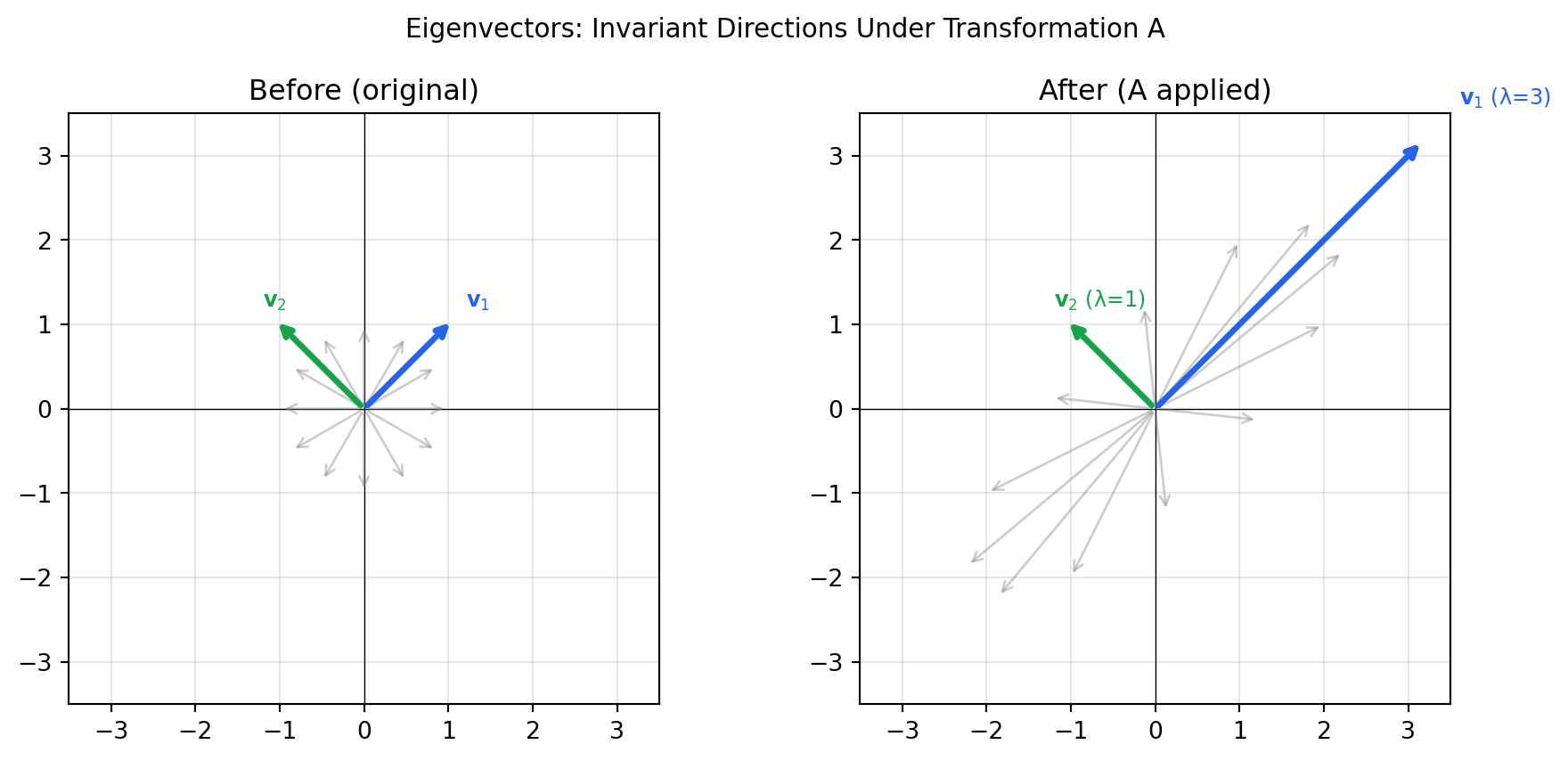
### Intuition
Most vectors change both direction and magnitude when multiplied by a matrix.
**Eigenvectors** are special — they only scale:
$$A\mathbf{v} = \lambda \mathbf{v}$$
Here $\mathbf{v}$ is the eigenvector and $\lambda$ is the corresponding eigenvalue.
Think of the matrix $A$ as a transformation: eigenvectors are the axes the
transformation stretches or compresses, and eigenvalues say by how much.
**Why this matters in OR:**
- The spectral radius determines the convergence rate of iterative solvers
- Eigenvalues of the Hessian determine whether an objective is convex
- Positive definite matrices (all eigenvalues $> 0$) guarantee convexity
**Why this matters in ML:**
- Principal Component Analysis (PCA) finds eigenvectors of the covariance matrix
- The largest eigenvalue governs gradient stability in neural networks
- Spectral clustering decomposes graph Laplacians via eigenvectors
### Computing Eigenvalues and Eigenvectors
```{python}
#| label: eigen-basics
A = np.array([[3, 1],
              [0, 2]], dtype=float)

eigenvalues, eigenvectors = np.linalg.eig(A)

print("Matrix A:")
print(A)
print(f"\nEigenvalues:  {eigenvalues}")
print(f"Eigenvectors (columns):\n{eigenvectors}")

# Verify: Av = λv  for first eigenpair
v0, lam0 = eigenvectors[:, 0], eigenvalues[0]
print(f"\nVerification for λ={lam0:.1f}:")
print(f"  Av  = {A @ v0}")
print(f"  λv  = {lam0 * v0}")
print(f"  Match: {np.allclose(A @ v0, lam0 * v0)}")
```
### Visualising Eigenvectors as Transformation Axes
```{python}
#| label: fig-eigenvectors
#| fig-cap: "Eigenvectors (blue/green arrows) are the only directions preserved under the matrix transformation A. Other vectors (grey) are rotated."
fig, axes = plt.subplots(1, 2, figsize=(10, 4.5))

A = np.array([[2, 1], [1, 2]], dtype=float)
eigenvalues, eigenvectors = np.linalg.eig(A)

for ax, title, transform in zip(axes, ["Before (original)", "After (A applied)"], [False, True]):
    # Random unit vectors
    np.random.seed(0)
    angles = np.linspace(0, 2 * np.pi, 12, endpoint=False)
    vecs = np.stack([np.cos(angles), np.sin(angles)], axis=1)

    for v in vecs:
        end = A @ v if transform else v
        ax.annotate("", xy=end, xytext=[0, 0],
                    arrowprops=dict(arrowstyle="->", color="grey", alpha=0.4, lw=1))

    # Eigenvectors
    for i, color in enumerate(["#2563eb", "#16a34a"]):
        ev = eigenvectors[:, i]
        end = (A @ ev) if transform else ev
        ax.annotate("", xy=end * 1.5, xytext=[0, 0],
                    arrowprops=dict(arrowstyle="->", color=color, lw=2.5))
        lbl = f"$\\mathbf{{v}}_{i+1}$" + (f" (λ={eigenvalues[i]:.0f})" if transform else "")
        ax.text(end[0] * 1.7, end[1] * 1.7, lbl, color=color, fontsize=9)

    ax.set_xlim(-3.5, 3.5); ax.set_ylim(-3.5, 3.5)
    ax.axhline(0, color="black", lw=0.5); ax.axvline(0, color="black", lw=0.5)
    ax.grid(True, alpha=0.3)
    ax.set_title(title)
    ax.set_aspect("equal")

plt.suptitle("Eigenvectors: Invariant Directions Under Transformation A", fontsize=11)
plt.tight_layout()
plt.show()
```
### Eigenvalues and Convexity
In optimisation, a function $f(\mathbf{x})$ is **convex** if its Hessian matrix
$H = \nabla^2 f$ is positive semi-definite everywhere — meaning all eigenvalues of
$H$ are $\geq 0$. This is crucial: convex problems have no local minima that are not
also global minima, which is what makes LP, QP, and convex programming tractable.
```{python}
#| label: hessian-convexity
# Hessian of f(x1, x2) = x1^2 + 2*x1*x2 + 3*x2^2  (a convex quadratic)
H_convex = np.array([[2, 2],
                     [2, 6]])

# Hessian of a non-convex function
H_nonconvex = np.array([[2,  4],
                         [4, -1]])

for label, H in [("Convex Hessian", H_convex), ("Non-convex Hessian", H_nonconvex)]:
    eigs = np.linalg.eigvalsh(H)   # eigvalsh for symmetric matrices
    print(f"{label}:")
    print(f"  Eigenvalues: {eigs}")
    print(f"  All ≥ 0 (positive semi-definite)? {all(eigs >= -1e-9)}\n")
```
---
## Singular Value Decomposition {#sec-svd}
### Definition
The Singular Value Decomposition (SVD) factors any matrix $A \in \mathbb{R}^{m \times n}$ as:
$$A = U \Sigma V^T$$
where:
- $U \in \mathbb{R}^{m \times m}$ — orthogonal matrix; columns are **left singular vectors** (output directions)
- $\Sigma \in \mathbb{R}^{m \times n}$ — diagonal matrix of **singular values** $\sigma_1 \geq \sigma_2 \geq \cdots \geq 0$
- $V \in \mathbb{R}^{n \times n}$ — orthogonal matrix; columns are **right singular vectors** (input directions)
SVD is one of the most important matrix factorisations in applied mathematics. It
reveals the "true geometry" of a matrix — which directions carry the most information,
and how much.
### SVD in Python
```{python}
#| label: svd-basics
# Design matrix: 5 customers × 3 features
np.random.seed(7)
X = np.random.randn(5, 3)
X[:, 2] = 0.9 * X[:, 0] + 0.1 * np.random.randn(5)   # feature 3 ≈ feature 1

U, sigma, Vt = np.linalg.svd(X, full_matrices=False)

print("Singular values:", np.round(sigma, 3))
print(f"  → Most variance captured by first 2 components")
print(f"  → Feature 3 near-redundant: σ₃ = {sigma[2]:.3f} (small)")

# Explained variance ratio (analogous to PCA)
explained = sigma**2 / np.sum(sigma**2)
print("\nExplained variance ratio:", np.round(explained, 3))
print(f"First 2 components explain {100*explained[:2].sum():.1f}% of variance")
```
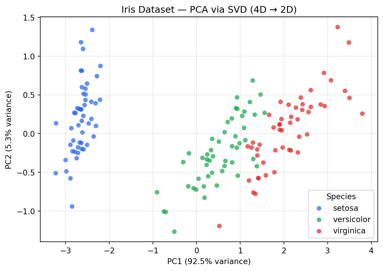
### PCA via SVD — Dimensionality Reduction
Principal Component Analysis (PCA) finds the directions of maximum variance in a
dataset. Computationally, it is exactly an SVD of the mean-centred data matrix.
This is the most widely used dimensionality-reduction technique in ML.
```{python}
#| label: fig-pca-svd
#| fig-cap: "PCA (via SVD) projects high-dimensional data onto the directions of maximum variance. Here, 4-feature data is reduced to 2 principal components."
from sklearn.decomposition import PCA
from sklearn.datasets import load_iris
import pandas as pd

iris = load_iris()
X_iris = iris.data          # 150 samples × 4 features
y_iris = iris.target

pca = PCA(n_components=2)
X_pca = pca.fit_transform(X_iris)

print("Original shape:", X_iris.shape)
print("Reduced shape: ", X_pca.shape)
print(f"Variance explained by PC1: {pca.explained_variance_ratio_[0]:.1%}")
print(f"Variance explained by PC2: {pca.explained_variance_ratio_[1]:.1%}")
print(f"Total (2 components):      {pca.explained_variance_ratio_.sum():.1%}")

# Plot
fig, ax = plt.subplots(figsize=(7, 5))
colors = ["#2563eb", "#16a34a", "#dc2626"]
for cls, color, name in zip([0, 1, 2], colors, iris.target_names):
    mask = y_iris == cls
    ax.scatter(X_pca[mask, 0], X_pca[mask, 1],
               c=color, label=name, alpha=0.7, edgecolors="none")

ax.set_xlabel(f"PC1 ({pca.explained_variance_ratio_[0]:.1%} variance)")
ax.set_ylabel(f"PC2 ({pca.explained_variance_ratio_[1]:.1%} variance)")
ax.set_title("Iris Dataset — PCA via SVD (4D → 2D)")
ax.legend(title="Species")
ax.grid(True, alpha=0.3)
plt.tight_layout()
plt.show()
```
---
## Linear Algebra in LP — Connecting Theory to Optimisation {#sec-lp-connection}
Every linear programme in standard form is fundamentally a linear algebra problem.
To see why, consider the LP:
$$\text{Minimize} \quad \mathbf{c}^T \mathbf{x} \qquad \text{subject to} \quad A\mathbf{x} = \mathbf{b},\ \mathbf{x} \geq 0$$
**The Simplex Method** navigates the vertices of the feasible polyhedron. At each
vertex, exactly $m$ constraints are active — selecting a **basis** $B$, a square
submatrix of $A$ that is invertible. The current solution is:
$$\mathbf{x}_B = B^{-1}\mathbf{b}$$
Moving to a better vertex means swapping one column into the basis and solving another
linear system. The entire Simplex algorithm is a sequence of matrix factorisations
and linear system solves — linear algebra all the way down.
```{python}
#| label: basis-demo
# Demonstrate the basis concept for a 2-constraint LP
# Maximize 40x_A + 30x_B  s.t.  4x_A + 2x_B <= 160,  2x_A + 3x_B <= 120

import pulp

model = pulp.LpProblem("LP_Basis_Demo", pulp.LpMaximize)
x_a = pulp.LpVariable("x_A", lowBound=0)
x_b = pulp.LpVariable("x_B", lowBound=0)

model += 40 * x_a + 30 * x_b
model += 4 * x_a + 2 * x_b <= 160, "machine"
model += 2 * x_a + 3 * x_b <= 120, "labour"

model.solve(pulp.PULP_CBC_CMD(msg=0))

x_opt = np.array([pulp.value(x_a), pulp.value(x_b)])
print(f"Optimal solution: x_A = {x_opt[0]:.2f}, x_B = {x_opt[1]:.2f}")

# At the optimum BOTH constraints are active — this defines the basis
A_basis = np.array([[4, 2],
                    [2, 3]])
b_rhs   = np.array([160.0, 120.0])

x_basis = np.linalg.solve(A_basis, b_rhs)
print(f"Basis solution (Bx = b): x_A = {x_basis[0]:.2f}, x_B = {x_basis[1]:.2f}")
print(f"Results match: {np.allclose(x_opt, x_basis)}")
print(f"\nBasic feasible solution: {x_basis}")
print(f"Objective value: ${40*x_basis[0] + 30*x_basis[1]:.2f}")
```
---
## Linear Algebra in ML — The Normal Equations {#sec-ml-connection}
Ordinary least squares regression has a closed-form solution rooted entirely in
linear algebra. Given design matrix $X \in \mathbb{R}^{N \times p}$ and targets
$\mathbf{y} \in \mathbb{R}^N$, the coefficients that minimise
$\|y - X\beta\|_2^2$ satisfy the **normal equations**:
$$X^T X \hat{\beta} = X^T \mathbf{y} \quad \Rightarrow \quad \hat{\beta} = (X^T X)^{-1} X^T \mathbf{y}$$
The matrix $X^T X$ is symmetric positive definite (when $X$ has full column rank),
guaranteeing a unique global minimum.
```{python}
#| label: normal-equations
np.random.seed(42)
N, p = 100, 3

# Generate synthetic dataset: y = 2*x1 + (-1)*x2 + 0.5*x3 + noise
beta_true = np.array([2.0, -1.0, 0.5])
X = np.random.randn(N, p)
y = X @ beta_true + np.random.randn(N) * 0.5

# Normal equations: β̂ = (X'X)^{-1} X'y
XtX = X.T @ X
Xty = X.T @ y
beta_hat = np.linalg.solve(XtX, Xty)   # solve, not invert

print(f"True coefficients:      {beta_true}")
print(f"Estimated coefficients: {np.round(beta_hat, 4)}")

# Compare to sklearn
from sklearn.linear_model import LinearRegression
lr = LinearRegression(fit_intercept=False).fit(X, y)
print(f"sklearn coefficients:   {np.round(lr.coef_, 4)}")

residuals = y - X @ beta_hat
print(f"\nR² = {1 - np.var(residuals)/np.var(y):.4f}")
```
---
## Chapter Summary {#sec-summary-linalg}
Linear algebra is not a preliminary formality — it is the computational substrate
on which all of OR and ML runs. The key ideas to carry forward:
- **Vectors** represent decisions, features, and gradients. The dot product is
the fundamental operation inside objective functions, constraints, and neural network
layers alike.
- **Matrices** encode transformations, constraints, and datasets. Matrix–vector
multiplication $A\mathbf{x}$ evaluates constraint satisfaction or applies a learned
transformation in a single operation.
- **Linear systems** $A\mathbf{x} = \mathbf{b}$ are solved at every step of the
Simplex Method and underpin the normal equations of linear regression.
- **Rank and invertibility** determine whether a system has a unique solution —
critical for LP optimality theory and for regression with correlated features.
- **Eigenvalues** reveal the shape of curvature (convexity), the convergence rate
of iterative algorithms, and the directions of maximum variance in data (PCA).
- **SVD** is the master factorisation: it underlies PCA, least-squares solvers,
recommender systems, and low-rank approximations used throughout ML.
- **The LP–linear algebra connection** is exact: solving an LP reduces to a sequence
of linear system solves over bases of the constraint matrix.
The next chapter, Probability and Statistics, adds the language of uncertainty —
giving us the tools to reason about stochastic demand, model error, and
decision-making under risk.