---
title: "Linear Programming"
subtitle: "Chapter 2 – Part II: Core Optimization Techniques"
author: "Troy Altus"
date: "2026-04-14"
number-sections: true
number-depth: 3
---
## What Is Linear Programming? {#sec-lp-intro}
Linear Programming (LP) is the foundation of Operations Research. It is the art — and
the science — of allocating scarce resources optimally when both the objective and the
constraints can be expressed as linear relationships.
The word *programming* here is a historical artifact meaning *planning*, not software.
When George Dantzig formulated LP in 1947 and invented the Simplex Method to solve it,
he gave practitioners their first general-purpose tool for large-scale optimization. That
tool remains, in modified form, at the core of virtually every commercial solver today.
LP problems appear under many names — resource allocation, production planning, diet
problems, blending problems, transportation problems — but they share a universal structure:
- A **linear objective function** to maximize or minimize
- A set of **linear inequality or equality constraints**
- **Non-negativity restrictions** on the decision variables
This chapter builds LP from the ground up: formulation, geometry, the Simplex Method,
duality, sensitivity analysis, and practical implementation in Python.
---
## Standard Form {#sec-standard-form}
Every LP can be written in **standard form**:
$$\text{Maximize} \quad \mathbf{c}^T \mathbf{x}$$
$$\text{subject to} \quad A\mathbf{x} \leq \mathbf{b}$$
$$\mathbf{x} \geq \mathbf{0}$$
Where:
- $\mathbf{x} \in \mathbb{R}^n$ — the vector of **decision variables**
- $\mathbf{c} \in \mathbb{R}^n$ — the **objective function coefficients** (profit, cost)
- $A \in \mathbb{R}^{m \times n}$ — the **constraint matrix**
- $\mathbf{b} \in \mathbb{R}^m$ — the **right-hand side** (resource limits)
Minimization problems are handled by negating the objective: $\min \mathbf{c}^T \mathbf{x}
= -\max (-\mathbf{c})^T \mathbf{x}$.
Equality constraints ($a_i^T \mathbf{x} = b_i$) can be introduced directly; most solvers
handle mixed forms natively.
### Formulating a Problem
Good LP formulation is a skill — the translation from prose to mathematics is rarely
mechanical. Three questions guide the process:
1. **What decisions need to be made?** → Define the decision variables.
2. **What do we want to achieve?** → Write the objective function.
3. **What limits our choices?** → Write the constraints.
A variable should represent something *controllable*. A constraint should represent
something *binding*. If you cannot write the problem in this form, LP may not be the
right tool.
---
## Geometric Intuition {#sec-geometry}
For problems with two decision variables, LP has a clean geometric interpretation that
reveals *why* the Simplex Method works.
Each linear inequality constraint defines a **half-plane** — the set of points on one
side of a line. The intersection of all half-planes (plus the non-negativity region) is
the **feasible region** — the set of all solutions that satisfy every constraint
simultaneously.
The objective function $Z = c_1 x_1 + c_2 x_2$ defines a family of parallel lines,
each corresponding to a different value of $Z$. Maximizing $Z$ means pushing this line
as far as possible in the direction of improvement while remaining inside the feasible
region.
The key theorem:
> **If an LP has an optimal solution, it occurs at a vertex (corner point) of the
> feasible region.**
This is a profound result. It means that even if the feasible region contains infinitely
many points, we only need to check a finite number of vertices to find the optimum.
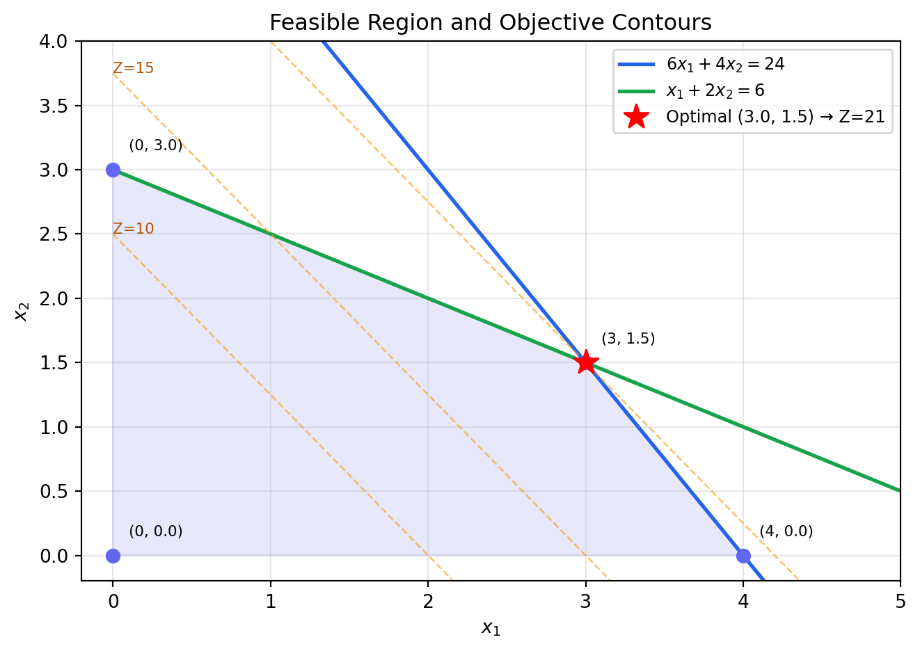
### Visualising the Feasible Region
```{python}
#| label: fig-feasible-region
#| fig-cap: "Feasible region and objective function contours for a two-variable LP"
import numpy as np
import matplotlib.pyplot as plt
import matplotlib.patches as mpatches
from matplotlib.lines import Line2D

# Problem:
#   Maximize  5x1 + 4x2
#   s.t.      6x1 + 4x2 <= 24
#             x1  + 2x2 <= 6
#             x1, x2    >= 0

fig, ax = plt.subplots(figsize=(7, 5))
x = np.linspace(0, 5, 400)

c1 = (24 - 6 * x) / 4   # 6x1 + 4x2 = 24
c2 = (6  - x)     / 2   # x1  + 2x2 = 6

ax.plot(x, c1, color="#2563eb", lw=2, label=r"$6x_1 + 4x_2 = 24$")
ax.plot(x, c2, color="#16a34a", lw=2, label=r"$x_1 + 2x_2 = 6$")

# Feasible region vertices
verts = np.array([[0, 0], [4, 0], [3, 1.5], [0, 3]])
ax.fill(verts[:, 0], verts[:, 1], alpha=0.15, color="#6366f1", zorder=1)

# Mark vertices
for v in verts:
    ax.plot(*v, "o", color="#6366f1", ms=7, zorder=3)
    ax.annotate(f"({v[0]:.0f}, {v[1]:.1f})", xy=v,
                xytext=(v[0] + 0.1, v[1] + 0.15), fontsize=8)

# Optimal point
opt = np.array([3, 1.5])
ax.plot(*opt, "r*", ms=14, zorder=4, label=f"Optimal (3.0, 1.5) → Z=21")

# Objective contours
for z in [10, 15, 21]:
    xc = np.linspace(0, 5, 200)
    yc = (z - 5 * xc) / 4
    ax.plot(xc, yc, "--", color="#f59e0b", alpha=0.6, lw=1)
    ax.annotate(f"Z={z}", xy=(xc[xc >= 0][0], yc[xc >= 0][0]),
                fontsize=8, color="#b45309")

ax.set_xlim(-0.2, 5)
ax.set_ylim(-0.2, 4)
ax.set_xlabel(r"$x_1$")
ax.set_ylabel(r"$x_2$")
ax.set_title("Feasible Region and Objective Contours")
ax.legend(fontsize=9)
ax.grid(True, alpha=0.3)
plt.tight_layout()
plt.show()
```
The dashed lines are **iso-profit contours** — all points along each dashed line produce
the same objective value. As we push the contour toward higher $Z$, the last point of
contact with the feasible region is the optimal vertex.
---
## The Simplex Method {#sec-simplex}
The geometric approach breaks down for problems with more than two variables — we cannot
visualise a 100-dimensional feasible region. The **Simplex Method** generalises the
vertex-search idea algebraically.
The algorithm starts at a feasible vertex and moves along edges of the feasible region
to an adjacent vertex with a better objective value. It repeats until no improving move
exists — at which point the current vertex is optimal.
### Basic Feasible Solutions
In algebraic terms, a **basic feasible solution** (BFS) corresponds to a vertex. To
convert inequality constraints to equalities, we introduce **slack variables**:
$$6x_1 + 4x_2 + s_1 = 24$$
$$x_1 + 2x_2 + s_2 = 6$$
A BFS sets $n$ variables to zero (the *non-basic* variables) and solves for the remaining
$m$ (the *basic* variables). In a two-constraint, two-variable problem this gives $\binom{4}{2} = 6$
candidate vertices — only those with all values $\geq 0$ are feasible.
### Entering and Leaving the Basis
At each iteration, the Simplex Method:
1. **Selects an entering variable** — the non-basic variable whose coefficient in the
objective row is most negative (for maximisation in standard minimisation tableau form).
2. **Performs a minimum ratio test** — identifies which basic variable reaches zero first
as the entering variable increases, determining the **leaving variable**.
3. **Pivots** — performs row operations to swap entering and leaving variables.
This continues until no entering variable can improve the objective — the optimality condition.
### Complexity
In the worst case, Simplex visits an exponential number of vertices. In practice, it is
remarkably efficient — typically solving problems with thousands of variables in seconds.
The **revised Simplex** and **interior-point** methods (e.g., Karmarkar's algorithm, 1984)
provide polynomial-time alternatives that modern solvers blend adaptively.
For practical purposes, we delegate solving to CBC (via PuLP) and focus on formulation
and interpretation.
---
## Python Implementation with PuLP {#sec-pulp}
PuLP provides a clean, readable interface for formulating and solving LP problems. The
workflow is consistent across all problem types.
### Case Study: Production Planning
A factory produces three products — **Chairs**, **Tables**, and **Shelves** — using two
shared resources: **wood** (board-feet) and **labour** (hours).
| Product | Wood (bf) | Labour (hr) | Profit ($) |
|---------|-----------|-------------|------------|
| Chair | 3 | 2 | 45 |
| Table | 5 | 4 | 80 |
| Shelf | 2 | 1 | 30 |
Weekly resource limits: **240 board-feet** of wood, **120 hours** of labour.
Market demand caps: at most **40 chairs**, **30 tables**, **50 shelves** per week.
**Formulation:**
Let $x_C$, $x_T$, $x_S$ be weekly production quantities.
$$\text{Maximize} \quad Z = 45x_C + 80x_T + 30x_S$$
$$\text{subject to:}$$
$$3x_C + 5x_T + 2x_S \leq 240 \quad \text{(wood)}$$
$$2x_C + 4x_T + x_S \leq 120 \quad \text{(labour)}$$
$$x_C \leq 40, \quad x_T \leq 30, \quad x_S \leq 50$$
$$x_C, x_T, x_S \geq 0$$
```{python}
#| label: production-lp
import pulp

# Model
model = pulp.LpProblem("Production_Planning", pulp.LpMaximize)

# Decision variables
xC = pulp.LpVariable("Chairs",  lowBound=0, upBound=40)
xT = pulp.LpVariable("Tables",  lowBound=0, upBound=30)
xS = pulp.LpVariable("Shelves", lowBound=0, upBound=50)

# Objective
model += 45 * xC + 80 * xT + 30 * xS, "Total_Profit"

# Resource constraints
wood_constraint   = 3 * xC + 5 * xT + 2 * xS <= 240
labour_constraint = 2 * xC + 4 * xT + xS      <= 120

model += wood_constraint,   "Wood"
model += labour_constraint, "Labour"

# Solve
model.solve(pulp.PULP_CBC_CMD(msg=0))

print(f"Status  : {pulp.LpStatus[model.status]}")
print(f"Chairs  : {pulp.value(xC):.1f} units/week")
print(f"Tables  : {pulp.value(xT):.1f} units/week")
print(f"Shelves : {pulp.value(xS):.1f} units/week")
print(f"Profit  : ${pulp.value(model.objective):,.2f}/week")
```
### Reading the Solution
The solver returns the **optimal production mix** — the combination that maximises
weekly profit without exceeding any resource limit. Notice that the market demand caps
on tables and shelves may or may not bind; the shadow prices (below) reveal which
constraints are actually limiting growth.
---
## Sensitivity Analysis {#sec-sensitivity}
An optimal solution answers *what* to do. Sensitivity analysis answers *how confident
we should be* in that answer and *where to focus improvement efforts*.
### Shadow Prices
The **shadow price** (or **dual value**) of a constraint measures how much the objective
would improve if that constraint's right-hand side were relaxed by one unit.
- Shadow price = 0 → constraint is **slack** (not binding); relaxing it changes nothing.
- Shadow price > 0 → constraint is **binding**; each additional unit of that resource is
worth exactly the shadow price in objective improvement.
```{python}
#| label: shadow-prices
print("Shadow Prices (dual values):")
print(f"  Wood   : ${model.constraints['Wood'].pi:.4f} per board-foot")
print(f"  Labour : ${model.constraints['Labour'].pi:.4f} per hour")

print("\nSlack (unused capacity):")
print(f"  Wood   : {-model.constraints['Wood'].slack:.1f} bf used of 240")
print(f"  Labour : {-model.constraints['Labour'].slack:.1f} hr used of 120")
```
### Reduced Costs
The **reduced cost** of a decision variable is the amount by which its objective
coefficient would need to improve before it would enter an optimal solution at a
positive level. Variables already in the solution have a reduced cost of zero.
```{python}
#| label: reduced-costs
print("Reduced Costs:")
for v in [xC, xT, xS]:
    print(f"  {v.name:8s}: {v.dj:.4f}")
```
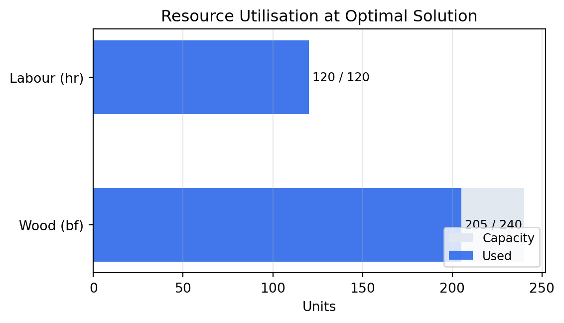
### Visualising Resource Utilisation
```{python}
#| label: fig-resource-utilisation
#| fig-cap: "Resource utilisation at the optimal solution"
import matplotlib.pyplot as plt

resources  = ["Wood (bf)", "Labour (hr)"]
capacity   = [240, 120]
used       = [
    3 * pulp.value(xC) + 5 * pulp.value(xT) + 2 * pulp.value(xS),
    2 * pulp.value(xC) + 4 * pulp.value(xT) +     pulp.value(xS),
]

fig, ax = plt.subplots(figsize=(6, 3.5))
x_pos = range(len(resources))

ax.barh(x_pos, capacity, color="#e2e8f0", height=0.5, label="Capacity")
ax.barh(x_pos, used,     color="#2563eb", height=0.5, alpha=0.85, label="Used")

for i, (u, c) in enumerate(zip(used, capacity)):
    ax.text(u + 2, i, f"{u:.0f} / {c}", va="center", fontsize=9)

ax.set_yticks(list(x_pos))
ax.set_yticklabels(resources)
ax.set_xlabel("Units")
ax.set_title("Resource Utilisation at Optimal Solution")
ax.legend(loc="lower right", fontsize=9)
ax.grid(axis="x", alpha=0.3)
plt.tight_layout()
plt.show()
```
A fully utilised resource (no slack) has a positive shadow price. An underutilised
resource has a shadow price of zero — acquiring more of it adds no value at the current
optimum.
---
## Duality {#sec-duality}
Every LP (the **primal**) has a companion problem called the **dual**. The dual offers
a different perspective on the same problem — and a powerful tool for understanding
what the solution means.
### Constructing the Dual
For a primal maximisation problem:
$$\text{Primal:} \quad \max\ \mathbf{c}^T \mathbf{x} \quad \text{s.t.}\ A\mathbf{x} \leq \mathbf{b},\ \mathbf{x} \geq \mathbf{0}$$
The dual is:
$$\text{Dual:} \quad \min\ \mathbf{b}^T \mathbf{y} \quad \text{s.t.}\ A^T \mathbf{y} \geq \mathbf{c},\ \mathbf{y} \geq \mathbf{0}$$
Where $\mathbf{y} \in \mathbb{R}^m$ are the **dual variables** — one per primal constraint.
### Economic Interpretation
The dual variables $y_i$ are precisely the **shadow prices** from the previous section.
They represent the **marginal value** of each resource: the maximum price a rational
firm should be willing to pay for one additional unit of resource $i$.
The dual constraint $A^T \mathbf{y} \geq \mathbf{c}$ says: the implicit value of the
resources consumed by each product must be at least as large as that product's profit.
If it were less, you could profitably buy more resources and produce more — contradicting
optimality.
### Strong Duality
The most important result in LP:
> **At optimality, the primal and dual objectives are equal:**
> $$\mathbf{c}^T \mathbf{x}^* = \mathbf{b}^T \mathbf{y}^*$$
This means the maximum profit equals the minimum total imputed resource value — every
unit of profit can be fully attributed to the resources that produced it.
---
## Special Cases {#sec-special}
### Infeasibility
A problem is **infeasible** if no point satisfies all constraints simultaneously. This
usually signals a modelling error — incompatible constraints, overly tight bounds, or
a missing variable. PuLP returns `"Infeasible"` and the objective value is undefined.
```{python}
#| label: infeasible-example
m = pulp.LpProblem("Infeasible_Demo", pulp.LpMaximize)
x = pulp.LpVariable("x", lowBound=0)
m += x
m += x >= 10
m += x <= 5
m.solve(pulp.PULP_CBC_CMD(msg=0))
print(f"Status: {pulp.LpStatus[m.status]}")  # Infeasible
```
### Unboundedness
A problem is **unbounded** if the objective can be improved without limit. This also
signals a model error — a missing constraint that should cap the objective. PuLP returns
`"Unbounded"`.
### Multiple Optima
When the objective function is parallel to a binding constraint, the optimal objective
value is achieved by an entire **edge** of the feasible region — infinitely many
solutions all with the same objective value. Solvers return one vertex, but any convex
combination of the degenerate vertices is also optimal.
---
## A Larger Example: Diet Optimisation {#sec-diet}
The **diet problem** — minimise cost while meeting nutritional requirements — is an OR
classic. Introduced by Stigler in 1945, it was one of the first practical LPs ever solved.
```{python}
#| label: diet-problem
import pulp
import pandas as pd

# Food options: (cost per serving $, protein g, carbs g, fat g, calories)
foods = {
    "Oats":        (0.30, 5,  27, 3,  150),
    "Eggs":        (0.25, 6,   1, 5,   70),
    "Chicken":     (1.20, 25,  0, 5,  165),
    "Broccoli":    (0.40, 3,   6, 0,   55),
    "Brown Rice":  (0.20, 3,  45, 1,  215),
    "Greek Yogurt":(0.60, 10,  7, 0,   59),
    "Almonds":     (0.50, 6,   6, 14,  164),
}

# Minimum daily requirements
min_protein  = 50   # g
min_carbs    = 130  # g
max_fat      = 65   # g
min_calories = 1800
max_calories = 2200

model = pulp.LpProblem("Diet_Optimisation", pulp.LpMinimize)

servings = {
    food: pulp.LpVariable(food.replace(" ", "_"), lowBound=0)
    for food in foods
}

# Objective: minimise cost
model += pulp.lpSum(foods[f][0] * servings[f] for f in foods), "Total_Cost"

# Nutritional constraints
model += pulp.lpSum(foods[f][1] * servings[f] for f in foods) >= min_protein,  "Protein"
model += pulp.lpSum(foods[f][2] * servings[f] for f in foods) >= min_carbs,    "Carbs"
model += pulp.lpSum(foods[f][3] * servings[f] for f in foods) <= max_fat,      "Fat"
model += pulp.lpSum(foods[f][4] * servings[f] for f in foods) >= min_calories, "Min_Cal"
model += pulp.lpSum(foods[f][4] * servings[f] for f in foods) <= max_calories, "Max_Cal"

model.solve(pulp.PULP_CBC_CMD(msg=0))

print(f"Status       : {pulp.LpStatus[model.status]}")
print(f"Daily cost   : ${pulp.value(model.objective):.2f}\n")
print("Optimal servings:")
for food, var in servings.items():
    qty = pulp.value(var)
    if qty and qty > 0.01:
        print(f"  {food:15s}: {qty:.2f} serving(s)")

# Nutritional totals
protein  = sum(foods[f][1] * pulp.value(servings[f]) for f in foods)
carbs    = sum(foods[f][2] * pulp.value(servings[f]) for f in foods)
fat      = sum(foods[f][3] * pulp.value(servings[f]) for f in foods)
calories = sum(foods[f][4] * pulp.value(servings[f]) for f in foods)

print(f"\nNutritional totals:")
print(f"  Protein  : {protein:.1f}g  (min {min_protein}g)")
print(f"  Carbs    : {carbs:.1f}g  (min {min_carbs}g)")
print(f"  Fat      : {fat:.1f}g  (max {max_fat}g)")
print(f"  Calories : {calories:.0f} kcal  ({min_calories}–{max_calories})")
```
The diet problem highlights a common LP characteristic: the optimal solution is often
**corner-heavy**, concentrating on a small number of foods. This is mathematically
correct but practically unappealing. In practice, additional constraints (variety limits,
maximum servings per food) or objective modifications introduce more realistic solutions.
---
## When LP Is and Is Not Appropriate {#sec-limits}
LP is the right tool when:
- The objective and all constraints are genuinely linear
- Decision variables can take any non-negative real value (fractional solutions are acceptable)
- The problem is deterministic — parameters are known
LP is the **wrong** tool when:
| Situation | Better approach |
|---|---|
| Decisions must be whole numbers (order 5 trucks, not 4.7) | Integer Programming (Chapter 3) |
| Objective or constraints are nonlinear (quadratic cost, diminishing returns) | Nonlinear Programming (Chapter 6) |
| Parameters are uncertain (demand varies stochastically) | Stochastic Programming (Chapter 5) |
| The problem involves sequential decisions over time | Dynamic Programming / RL (Chapter 9) |
Recognising which tool fits which problem is the core skill of an OR practitioner.
---
## Chapter Summary {#sec-lp-summary}
- Linear Programming optimises a linear objective subject to linear constraints — the
foundational model in Operations Research
- The feasible region is a convex polyhedron; optimal solutions always occur at vertices
- The **Simplex Method** searches vertices efficiently by moving along improving edges
- **Shadow prices** quantify the marginal value of each constrained resource and guide
investment decisions
- **Duality** links every maximisation problem to a companion minimisation problem; at
optimality, their objectives are equal
- PuLP provides a clean Python interface for formulating, solving, and interrogating LP
models via the CBC solver
- LP is appropriate when the model is linear and decision variables are continuous;
integrality, nonlinearity, or uncertainty require different methods