---
title: "Network Optimization"
subtitle: "Chapter 4 – Part II: Core Optimization Techniques"
author: "Troy Altus"
date: "2026-04-14"
number-sections: true
number-depth: 3
---
## Networks Are Everywhere {#sec-net-intro}
A network is a set of **nodes** connected by **edges**. That simple structure models
an enormous range of real-world systems:
- Road and rail networks — nodes are intersections, edges are roads
- Supply chains — nodes are factories, warehouses, and retailers; edges are shipping lanes
- Telecommunications — nodes are routers, edges are fibre links
- Social networks — nodes are people, edges are relationships
- Project schedules — nodes are tasks, edges are dependencies
Network Optimization exploits the structure of these problems to solve them far more
efficiently than general-purpose LP or IP methods. The two key tools are **graph theory**
(representing structure) and **network flow** (optimising over that structure).
Python's `networkx` library provides the data structures; `pulp` provides the
optimisation. Together they handle problems from shortest paths to minimum cost flows.
---
## Graph Fundamentals {#sec-graphs}
A **graph** $G = (V, E)$ consists of:
- $V$ — a set of **vertices** (nodes)
- $E$ — a set of **edges** (arcs), where each edge connects two vertices
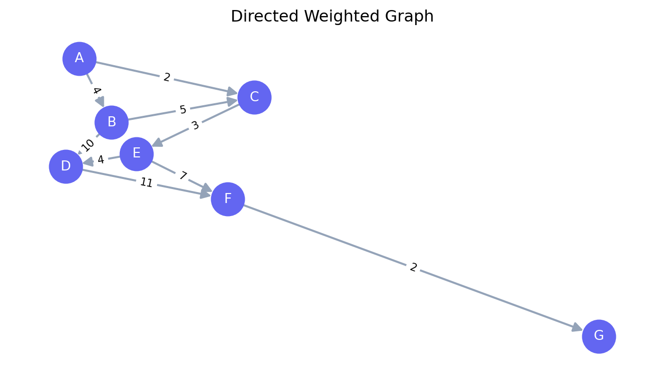
**Directed graphs (digraphs)** have edges with a direction — from a *tail* node to
a *head* node. Flow on an arc moves in one direction only.
**Undirected graphs** have edges with no direction — you can traverse them either way.
Key properties:
| Term | Definition |
|---|---|
| **Degree** | Number of edges incident to a node |
| **Path** | Sequence of edges connecting two nodes without repeating nodes |
| **Cycle** | A path that starts and ends at the same node |
| **Connected** | Every pair of nodes has at least one path between them |
| **Tree** | A connected graph with no cycles ($\|E\| = \|V\| - 1$) |
| **Spanning tree** | A tree that includes all nodes of the graph |
```{python}
#| label: fig-graph-basics
#| fig-cap: "A directed weighted graph"
import networkx as nx
import matplotlib.pyplot as plt

G = nx.DiGraph()
edges = [
    ("A", "B", 4), ("A", "C", 2), ("B", "C", 5),
    ("B", "D", 10), ("C", "E", 3), ("D", "F", 11),
    ("E", "D", 4), ("E", "F", 7), ("F", "G", 2)
]
G.add_weighted_edges_from(edges)

pos = nx.spring_layout(G, seed=42)
weights = nx.get_edge_attributes(G, "weight")

fig, ax = plt.subplots(figsize=(7, 4))
nx.draw_networkx(G, pos, ax=ax, node_color="#6366f1", node_size=600,
                 font_color="white", font_size=10, arrows=True,
                 arrowsize=15, edge_color="#94a3b8", width=1.5)
nx.draw_networkx_edge_labels(G, pos, edge_labels=weights, font_size=8, ax=ax)
ax.set_title("Directed Weighted Graph")
ax.axis("off")
plt.tight_layout()
plt.show()
```
---
## Shortest Path {#sec-shortest-path}
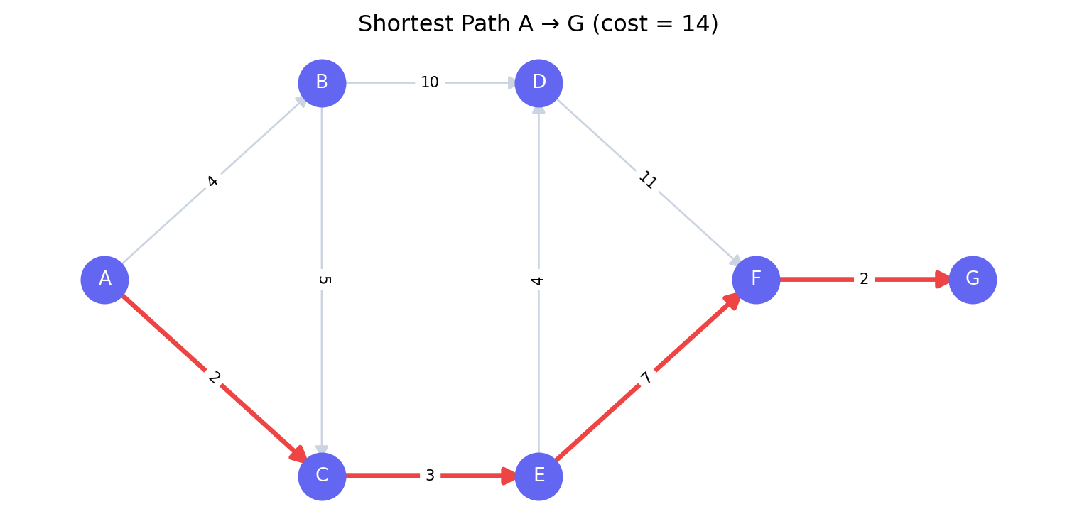
**Problem:** Find the minimum-cost path from a source node $s$ to a destination node
$t$ in a weighted graph.
**Applications:** GPS routing, network packet delivery, project critical path.
### Dijkstra's Algorithm
For graphs with non-negative edge weights, **Dijkstra's algorithm** finds shortest paths
from a single source in $O((V + E) \log V)$ time. It maintains a priority queue of
nodes ordered by their current shortest distance from the source, greedily expanding
the closest unvisited node at each step.
```{python}
#| label: shortest-path
import networkx as nx

G = nx.DiGraph()
edges = [
    ("A", "B", 4), ("A", "C", 2), ("B", "C", 5),
    ("B", "D", 10), ("C", "E", 3), ("D", "F", 11),
    ("E", "D", 4), ("E", "F", 7), ("F", "G", 2)
]
G.add_weighted_edges_from(edges)

path   = nx.dijkstra_path(G, "A", "G", weight="weight")
length = nx.dijkstra_path_length(G, "A", "G", weight="weight")

print(f"Shortest path : {' → '.join(path)}")
print(f"Total cost    : {length}")
```
### Visualising the Shortest Path
```{python}
#| label: fig-shortest-path
#| fig-cap: "Shortest path from A to G highlighted in red"
import matplotlib.pyplot as plt

pos = {"A": (0,1), "B": (1,2), "C": (1,0), "D": (2,2),
       "E": (2,0), "F": (3,1), "G": (4,1)}

path_edges = list(zip(path[:-1], path[1:]))
non_path   = [(u, v) for u, v, _ in edges if (u, v) not in path_edges]
weights    = nx.get_edge_attributes(G, "weight")

fig, ax = plt.subplots(figsize=(8, 4))
nx.draw_networkx_nodes(G, pos, node_color="#6366f1", node_size=600, ax=ax)
nx.draw_networkx_labels(G, pos, font_color="white", font_size=10, ax=ax)
nx.draw_networkx_edges(G, pos, edgelist=non_path, edge_color="#cbd5e1",
                       arrows=True, arrowsize=15, ax=ax)
nx.draw_networkx_edges(G, pos, edgelist=path_edges, edge_color="#ef4444",
                       width=2.5, arrows=True, arrowsize=18, ax=ax)
nx.draw_networkx_edge_labels(G, pos, edge_labels=weights, font_size=8, ax=ax)
ax.set_title(f"Shortest Path A → G (cost = {length})")
ax.axis("off")
plt.tight_layout()
plt.show()
```
### Bellman-Ford for Negative Weights
Dijkstra fails on graphs with negative edge weights. **Bellman-Ford** handles them in
$O(VE)$ time and also detects **negative cycles** (cycles where the total weight is
negative — the "shortest path" would be infinitely short by cycling forever).
```{python}
#| label: bellman-ford
G_neg = nx.DiGraph()
G_neg.add_weighted_edges_from([
    ("S", "A", 6), ("S", "B", 7), ("A", "B", 8), ("A", "C", -4),
    ("B", "C", -3), ("B", "D", 9), ("C", "D", 7), ("D", "A", 2)
])

try:
    path_bf   = nx.bellman_ford_path(G_neg, "S", "D", weight="weight")
    length_bf = nx.bellman_ford_path_length(G_neg, "S", "D", weight="weight")
    print(f"Bellman-Ford path   : {' → '.join(path_bf)}")
    print(f"Total cost          : {length_bf}")
except nx.exception.NetworkXUnbounded:
    print("Negative cycle detected — shortest path is undefined")
```
---
## Minimum Spanning Tree {#sec-mst}
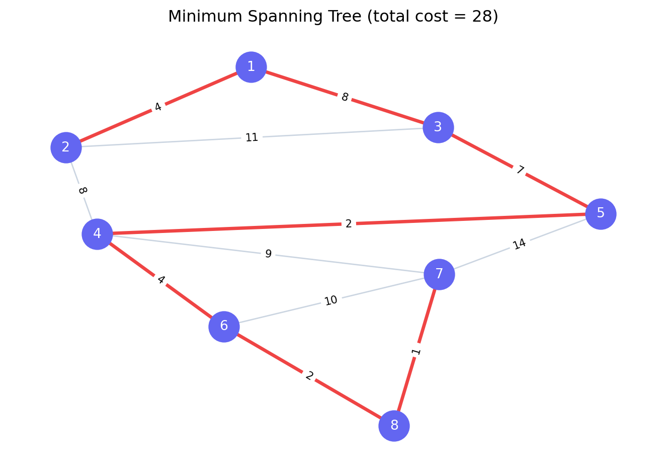
**Problem:** Connect all nodes in an undirected graph with the minimum total edge weight,
using exactly $|V| - 1$ edges (a tree).
**Applications:** Network cable layout, cluster analysis, approximation algorithms for TSP.
Two classic algorithms:
- **Kruskal's** — sort edges by weight; add the cheapest edge that does not create a cycle
- **Prim's** — grow a tree from a seed node by repeatedly adding the cheapest edge
connecting the tree to a new node
Both run in $O(E \log E)$ for typical implementations.
```{python}
#| label: fig-mst
#| fig-cap: "Minimum Spanning Tree highlighted in red"
import networkx as nx
import matplotlib.pyplot as plt

G_und = nx.Graph()
G_und.add_weighted_edges_from([
    (1,2,4),(1,3,8),(2,3,11),(2,4,8),(3,5,7),(4,5,2),
    (4,6,4),(4,7,9),(5,7,14),(6,7,10),(6,8,2),(7,8,1)
])

mst      = nx.minimum_spanning_tree(G_und, weight="weight")
mst_cost = sum(d["weight"] for _, _, d in mst.edges(data=True))

pos       = nx.spring_layout(G_und, seed=0)
mst_edges = list(mst.edges())
non_mst   = [(u, v) for u, v in G_und.edges() if (u,v) not in mst_edges and (v,u) not in mst_edges]
all_weights = nx.get_edge_attributes(G_und, "weight")

fig, ax = plt.subplots(figsize=(7, 5))
nx.draw_networkx_nodes(G_und, pos, node_color="#6366f1", node_size=500, ax=ax)
nx.draw_networkx_labels(G_und, pos, font_color="white", font_size=10, ax=ax)
nx.draw_networkx_edges(G_und, pos, edgelist=non_mst, edge_color="#cbd5e1", ax=ax)
nx.draw_networkx_edges(G_und, pos, edgelist=mst_edges,
                       edge_color="#ef4444", width=2.5, ax=ax)
nx.draw_networkx_edge_labels(G_und, pos, edge_labels=all_weights, font_size=8, ax=ax)
ax.set_title(f"Minimum Spanning Tree (total cost = {mst_cost})")
ax.axis("off")
plt.tight_layout()
plt.show()
```
---
## Maximum Flow {#sec-max-flow}
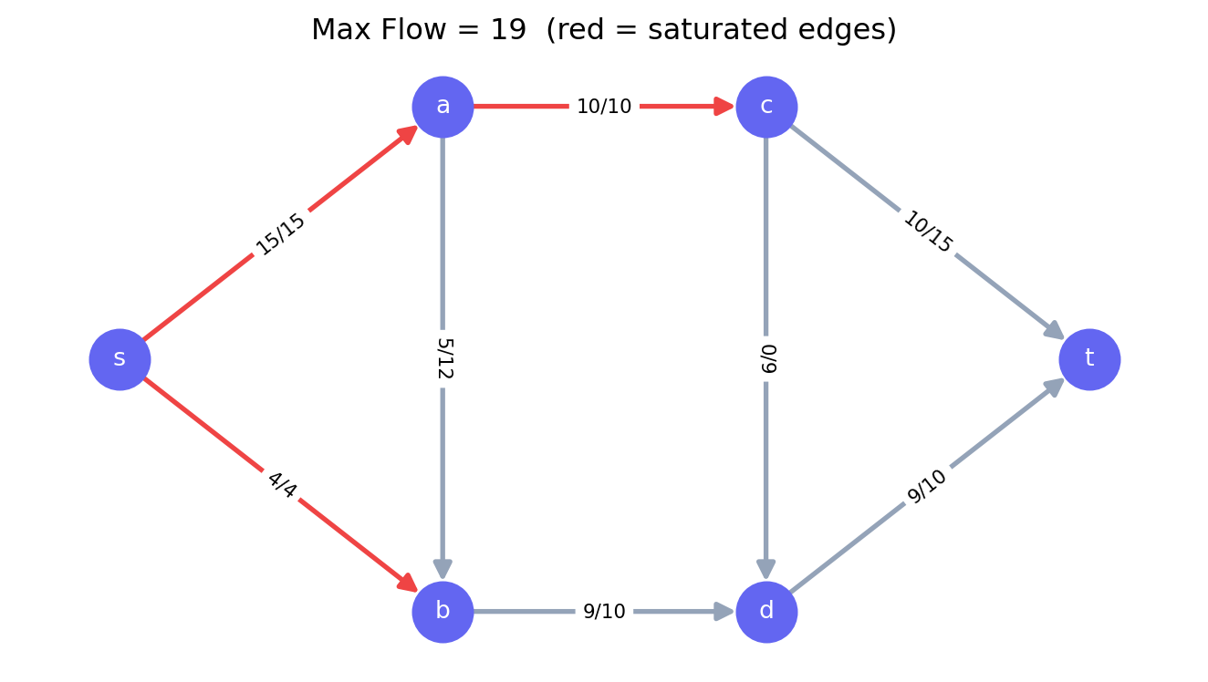
**Problem:** Given a directed graph with edge capacities, find the maximum amount of
flow that can be sent from a **source** $s$ to a **sink** $t$ without exceeding any
edge capacity.
**Applications:** Pipeline capacity, internet bandwidth allocation, bipartite matching.
### The Max-Flow Min-Cut Theorem
The maximum flow from $s$ to $t$ equals the minimum **cut** — the minimum total capacity
of edges that, if removed, would disconnect $s$ from $t$.
This duality is one of the most elegant results in combinatorial optimisation. It says
that the bottleneck in a network is always a cut — a set of edges that, collectively,
limits all paths from source to sink.
```{python}
#| label: max-flow
import networkx as nx

G_flow = nx.DiGraph()
G_flow.add_edge("s", "a", capacity=15)
G_flow.add_edge("s", "b", capacity=4)
G_flow.add_edge("a", "b", capacity=12)
G_flow.add_edge("a", "c", capacity=10)
G_flow.add_edge("b", "d", capacity=10)
G_flow.add_edge("c", "d", capacity=9)
G_flow.add_edge("c", "t", capacity=15)
G_flow.add_edge("d", "t", capacity=10)

flow_value, flow_dict = nx.maximum_flow(G_flow, "s", "t")

print(f"Maximum flow: {flow_value}")
print("\nFlow on each edge:")
for u in flow_dict:
    for v, f in flow_dict[u].items():
        if f > 0:
            cap = G_flow[u][v]["capacity"]
            print(f"  {u} → {v}: {f} / {cap}")
```
### Visualising Flow
```{python}
#| label: fig-max-flow
#| fig-cap: "Maximum flow network — edge labels show flow/capacity"
import matplotlib.pyplot as plt

pos = {"s": (0,1), "a": (1,2), "b": (1,0), "c": (2,2), "d": (2,0), "t": (3,1)}

edge_labels = {
    (u, v): f"{flow_dict[u].get(v, 0)}/{G_flow[u][v]['capacity']}"
    for u, v in G_flow.edges()
}
edge_colors = [
    "#ef4444" if flow_dict[u].get(v, 0) == G_flow[u][v]["capacity"] else "#94a3b8"
    for u, v in G_flow.edges()
]

fig, ax = plt.subplots(figsize=(7, 4))
nx.draw_networkx(G_flow, pos, ax=ax, node_color="#6366f1", node_size=600,
                 font_color="white", font_size=10, arrows=True,
                 arrowsize=15, edge_color=edge_colors, width=2)
nx.draw_networkx_edge_labels(G_flow, pos, edge_labels=edge_labels,
                              font_size=8, ax=ax)
ax.set_title(f"Max Flow = {flow_value}  (red = saturated edges)")
ax.axis("off")
plt.tight_layout()
plt.show()
```
Saturated edges (flow = capacity, shown in red) form the **minimum cut** — these are
the bottlenecks limiting total throughput.
---
## Minimum Cost Flow {#sec-min-cost-flow}
**Minimum Cost Flow (MCF)** is the most general network flow problem. It subsumes
shortest path, max flow, transportation, and assignment problems as special cases.
**Formulation:** Each arc $(i,j)$ has a **capacity** $u_{ij}$, a **lower bound**
$l_{ij}$, and a **unit cost** $c_{ij}$. Each node has a **supply** $b_i$ (positive
if it generates flow, negative if it consumes flow, zero if it is a transshipment node).
$$\text{Minimize} \quad \sum_{(i,j) \in E} c_{ij} x_{ij}$$
$$\text{s.t.} \quad \sum_{j:(i,j)\in E} x_{ij} - \sum_{j:(j,i)\in E} x_{ji} = b_i \quad \forall i \in V \quad \text{(flow balance)}$$
$$l_{ij} \leq x_{ij} \leq u_{ij} \quad \forall (i,j) \in E$$
The flow balance constraint says: flow out minus flow in equals supply at each node.
Supply nodes ($b_i > 0$) generate flow; demand nodes ($b_i < 0$) absorb it.
```{python}
#| label: min-cost-flow
import pulp

# Three suppliers (S1, S2, S3), three customers (C1, C2, C3), two warehouses (W1, W2)
# Cost per unit on each arc, capacity, supply/demand

nodes = ["S1", "S2", "S3", "W1", "W2", "C1", "C2", "C3"]

supply = {"S1": 120, "S2": 80,  "S3": 100,
          "W1": 0,   "W2": 0,
          "C1": -90, "C2": -110, "C3": -100}

arcs = {
    ("S1", "W1"): (8,  120), ("S1", "W2"): (6,  120),
    ("S2", "W1"): (5,  80),  ("S2", "W2"): (9,  80),
    ("S3", "W1"): (7,  100), ("S3", "W2"): (4,  100),
    ("W1", "C1"): (3,  200), ("W1", "C2"): (5,  200), ("W1", "C3"): (6,  200),
    ("W2", "C1"): (7,  200), ("W2", "C2"): (2,  200), ("W2", "C3"): (4,  200),
}  # (cost, capacity)

model = pulp.LpProblem("Min_Cost_Flow", pulp.LpMinimize)

x = {(i, j): pulp.LpVariable(f"x_{i}_{j}", lowBound=0, upBound=cap)
     for (i, j), (_, cap) in arcs.items()}

# Objective
model += pulp.lpSum(cost * x[i, j] for (i, j), (cost, _) in arcs.items())

# Flow balance
for node in nodes:
    out_flow = pulp.lpSum(x[i, j] for (i, j) in arcs if i == node)
    in_flow  = pulp.lpSum(x[i, j] for (i, j) in arcs if j == node)
    model += out_flow - in_flow == supply[node], f"Balance_{node}"

model.solve(pulp.PULP_CBC_CMD(msg=0))

print(f"Status      : {pulp.LpStatus[model.status]}")
print(f"Total cost  : ${pulp.value(model.objective):,.0f}\n")
print("Flow routing:")
for (i, j), var in x.items():
    flow = pulp.value(var)
    if flow and flow > 0.01:
        print(f"  {i} → {j}: {flow:.0f} units")
```
MCF is solvable in polynomial time using the **network simplex algorithm** — a
specialised version of the Simplex Method that exploits the tree structure of
network flow bases. It is typically orders of magnitude faster than general LP for
network problems.
---
## The Transportation Problem {#sec-transportation}
The **transportation problem** is a special case of MCF with a bipartite structure:
$m$ supply nodes and $n$ demand nodes, all connected directly (no intermediate
transshipment nodes).
It models the classic question: *how to ship goods from warehouses to customers at
minimum cost, given supply and demand constraints?*
```{python}
#| label: transportation
import pulp
import numpy as np
import matplotlib.pyplot as plt

# 3 suppliers, 4 customers
supply   = [300, 400, 500]
demand   = [250, 350, 400, 200]
cost_mat = np.array([
    [2, 3, 1, 5],
    [7, 3, 4, 2],
    [6, 1, 3, 4],
])

n_sup = len(supply)
n_dem = len(demand)

model = pulp.LpProblem("Transportation", pulp.LpMinimize)

x = [[pulp.LpVariable(f"x_{i}_{j}", lowBound=0)
      for j in range(n_dem)] for i in range(n_sup)]

# Objective
model += pulp.lpSum(cost_mat[i, j] * x[i][j]
                    for i in range(n_sup) for j in range(n_dem))

# Supply constraints
for i in range(n_sup):
    model += pulp.lpSum(x[i][j] for j in range(n_dem)) <= supply[i], f"Supply_{i}"

# Demand constraints
for j in range(n_dem):
    model += pulp.lpSum(x[i][j] for i in range(n_sup)) == demand[j], f"Demand_{j}"

model.solve(pulp.PULP_CBC_CMD(msg=0))

print(f"Status     : {pulp.LpStatus[model.status]}")
print(f"Total cost : ${pulp.value(model.objective):,.0f}\n")

print("Shipment plan (units):")
header = "         " + "  ".join(f"Cust {j+1:1d}" for j in range(n_dem))
print(header)
for i in range(n_sup):
    row = f"Supplier {i+1}: " + "  ".join(
        f"{pulp.value(x[i][j]):6.0f}" for j in range(n_dem)
    )
    print(row)
```
---
## Project Scheduling: CPM {#sec-cpm}
The **Critical Path Method (CPM)** applies shortest/longest path algorithms to project
scheduling. Activities are represented as edges (or nodes), with durations as weights.
The **critical path** is the longest path through the network — it determines the
minimum project duration.
Any delay on the critical path delays the entire project. Activities not on the critical
path have **float** (slack) — they can be delayed without affecting the project deadline.
```{python}
#| label: cpm
import networkx as nx
import matplotlib.pyplot as plt

# Activities: (predecessor, successor, duration)
activities = [
    ("START", "A", 0), ("START", "B", 0), ("START", "C", 0),
    ("A", "D", 3), ("A", "E", 3),
    ("B", "E", 5), ("B", "F", 5),
    ("C", "G", 2),
    ("D", "END", 4), ("E", "END", 6), ("F", "END", 2), ("G", "END", 7)
]

G = nx.DiGraph()
for pred, succ, dur in activities:
    G.add_edge(pred, succ, duration=dur)

# Longest path = critical path
critical_length = nx.dag_longest_path_length(G, weight="duration")
critical_path   = nx.dag_longest_path(G, weight="duration")

print(f"Project duration : {critical_length} days")
print(f"Critical path    : {' → '.join(critical_path)}")

# Early start times via topological sort
topo_order  = list(nx.topological_sort(G))
early_start = {node: 0 for node in G.nodes()}
for node in topo_order:
    for succ in G.successors(node):
        dur = G[node][succ]["duration"]
        early_start[succ] = max(early_start[succ], early_start[node] + dur)

print("\nEarly start times:")
for node, es in sorted(early_start.items(), key=lambda x: x[1]):
    print(f"  {node:6s}: day {es}")
```
The critical path tells a project manager exactly where to focus resources. Crashing
(accelerating) a non-critical activity wastes money; crashing a critical activity
directly reduces project duration.
---
## Choosing the Right Algorithm {#sec-algorithm-choice}
| Problem | Algorithm | Complexity |
|---|---|---|
| Single-source shortest path (non-negative weights) | Dijkstra | $O((V+E)\log V)$ |
| Single-source shortest path (negative weights) | Bellman-Ford | $O(VE)$ |
| All-pairs shortest path | Floyd-Warshall | $O(V^3)$ |
| Minimum spanning tree | Kruskal / Prim | $O(E \log E)$ |
| Maximum flow | Ford-Fulkerson / Push-relabel | $O(VE^2)$ |
| Minimum cost flow | Network Simplex | $O(VE \log V \log(VC))$ |
| Transportation | Simplex (network form) | Fast in practice |
| Bipartite matching | Hungarian algorithm | $O(V^3)$ |
For most practical problems, `networkx` and `pulp` provide sufficient performance.
For large-scale production systems (millions of nodes), Google OR-Tools' network flow
solver or Gurobi's built-in network simplex are preferred.
---
## Chapter Summary {#sec-net-summary}
- Network Optimization models systems as graphs (nodes and edges) and finds optimal
routes, flows, or spanning structures
- **Shortest path** (Dijkstra, Bellman-Ford) solves routing and scheduling problems;
the critical path in project management is the longest-path analogue
- **Minimum spanning tree** (Kruskal, Prim) connects all nodes at minimum total edge
cost — used in network design and cluster analysis
- **Maximum flow** (Ford-Fulkerson) finds the throughput limit of a network; by the
Max-Flow Min-Cut theorem, this equals the minimum cut capacity
- **Minimum cost flow** is the most general network model, subsuming transportation,
assignment, and shortest path as special cases
- Python's `networkx` provides graph data structures and classical algorithms; `pulp`
solves formulated network problems as LP/MIP
- Network algorithms exploit problem structure to achieve dramatically better
performance than general LP solvers on the same problems