---
title: "Introduction to Operations Research and Machine Learning"
number-sections: true
number-depth: 3
---
## What Is Operations Research? {#sec-what-is-or}
Operations Research (OR) is the scientific discipline concerned with the application of
analytical methods to improve decision-making. Born out of military logistics problems
during World War II, OR has grown into a broad field spanning industries from
manufacturing and supply chain to finance, healthcare, and transportation.
At its core, OR asks a deceptively simple question: **given limited resources and
competing objectives, what is the best possible decision?**
The answer requires translating real-world problems into mathematical models, solving
those models with rigorous algorithms, and interpreting the results in actionable terms.
### The Decision-Making Framework
Every OR problem shares a common structure:
- **Decision variables** — the quantities we control
- **Objective function** — the metric we want to optimize (minimize cost, maximize profit)
- **Constraints** — the limits within which decisions must operate
- **Parameters** — the known data that defines the problem
This structure is not merely academic. It forces clarity: you cannot optimize what you
have not defined, and you cannot define it without understanding the system.
### A Brief History
OR emerged formally in the 1940s when Allied forces assembled interdisciplinary teams —
mathematicians, physicists, engineers — to solve operational problems: how to route
convoys to minimize losses, how to allocate radar resources, how to schedule bombing
missions. The success of these teams demonstrated that quantitative methods could
outperform intuition at scale.
After the war, OR migrated into industry. George Dantzig's development of the **Simplex
Method** in 1947 gave practitioners the first general-purpose algorithm for linear
optimization. The following decades brought integer programming, network flows, dynamic
programming, and stochastic methods — each expanding the range of problems OR could address.
Today, OR sits at the foundation of every major logistics platform, airline scheduling
system, financial risk model, and supply chain optimizer in the world.
---
## What Is Machine Learning? {#sec-what-is-ml}
Machine Learning (ML) is the field of building systems that learn patterns from data
and use those patterns to make predictions or decisions — without being explicitly
programmed with rules.
Where OR starts with a model defined by human expertise, ML starts with data and
discovers structure automatically. Where OR optimizes a known objective, ML often
constructs the objective itself from observed outcomes.
### The Learning Paradigm
ML problems fall into three broad categories:
**Supervised Learning** trains a model on labeled examples — inputs paired with known
outputs — and learns to predict outputs for new inputs. Predicting equipment failure
from sensor readings, or estimating customer lifetime value from transaction history,
are supervised problems.
**Unsupervised Learning** finds structure in unlabeled data. Clustering customers by
purchasing behavior, or detecting anomalies in network traffic, requires no predefined
labels — only the data itself.
**Reinforcement Learning** trains an agent to take actions in an environment by
rewarding good outcomes and penalizing bad ones. It is the learning paradigm most
naturally aligned with OR's sequential decision-making problems.
### The Role of Data
ML's power is inseparable from data. More data, more representative data, and
better-quality data consistently produce better models. This dependence is also ML's
principal limitation: models trained on historical data can fail when the world changes,
and patterns learned from biased data reproduce that bias at scale.
Understanding these limitations is as important as understanding the methods themselves.
---
## The Intersection: OR Meets ML {#sec-intersection}
For decades, OR and ML developed largely in parallel — OR in engineering and management
science departments, ML in computer science and statistics. The two fields share deep
mathematical roots (linear algebra, probability, optimization) but developed distinct
cultures, vocabularies, and toolkits.
That separation is dissolving. Three forces are driving convergence:
**Scale.** Modern OR problems — routing millions of packages, pricing billions of
airline seats, scheduling thousands of employees — generate data volumes that dwarf
what any expert model can absorb. ML provides the tools to extract signal from that data.
**Uncertainty.** Classical OR models assume parameters are known. Real decisions happen
under uncertainty: demand fluctuates, travel times vary, equipment fails. ML offers
principled ways to estimate distributions and quantify uncertainty from data.
**Complexity.** Some systems are too complex to model from first principles. When the
physics of a supply chain or a financial market resist closed-form description, ML can
approximate the system well enough to optimize against.
### Where Each Method Excels
| Dimension | Operations Research | Machine Learning |
|---|---|---|
| Problem type | Optimization, scheduling, routing | Prediction, classification, pattern recognition |
| Data requirement | Low — model-driven | High — data-driven |
| Interpretability | High — explicit model | Variable — often opaque |
| Optimality guarantee | Yes (for many problem classes) | No |
| Handles uncertainty | Via stochastic methods | Natively, from data |
| Scalability | Solver-dependent | Generally high |
Neither approach dominates. The most powerful modern systems combine both: ML predicts
demand, OR optimizes supply. ML estimates risk, OR allocates capital. ML identifies
anomalies, OR schedules responses.
### The Prescriptive Analytics Stack
A useful way to frame the OR-ML relationship is through the analytics maturity stack:
- **Descriptive analytics** — what happened? (statistics, dashboards)
- **Diagnostic analytics** — why did it happen? (root cause, attribution)
- **Predictive analytics** — what will happen? (**ML**)
- **Prescriptive analytics** — what should we do about it? (**OR**)
ML and OR together form the top two levels of this stack — the levels that translate
data into decisions.
---
## Python as the Unified Platform {#sec-python}
Python has become the dominant language for both OR and ML — not because it is the
fastest language (it is not), but because it offers the richest ecosystem of libraries,
the most readable syntax, and the broadest community of practitioners.
### Core Libraries Used in This Book
**Optimization**
- `PuLP` — linear and integer programming with multiple solver backends
- `scipy.optimize` — nonlinear optimization, root finding, curve fitting
- `cvxpy` — convex optimization with a disciplined modeling interface
- `networkx` — graph construction and network flow algorithms
**Machine Learning**
- `scikit-learn` — classification, regression, clustering, model selection
- `numpy` / `pandas` — numerical computation and data manipulation
- `matplotlib` / `seaborn` — visualization
**Simulation & Stochastics**
- `simpy` — discrete-event simulation
- `scipy.stats` — probability distributions and statistical testing
### Environment Setup
```{python}
#| label: setup
#| code-fold: false
# Verify core dependencies are available
import importlib

libraries = [
    "pulp",
    "scipy",
    "cvxpy",
    "networkx",
    "sklearn",
    "numpy",
    "pandas",
    "matplotlib",
    "simpy",
]

for lib in libraries:
    try:
        importlib.import_module(lib)
        print(f"  ✓  {lib}")
    except ImportError:
        print(f"  ✗  {lib}  <-- install required")
```
If any libraries show `✗`, install them with:
```bash
pip install pulp scipy cvxpy networkx scikit-learn numpy pandas matplotlib simpy
```
---
## A First OR Problem in Python {#sec-first-problem}
Before introducing any theory, let's build and solve a complete optimization problem
from scratch. This example establishes the pattern that every chapter in this book
will follow: formulate, implement, solve, interpret.
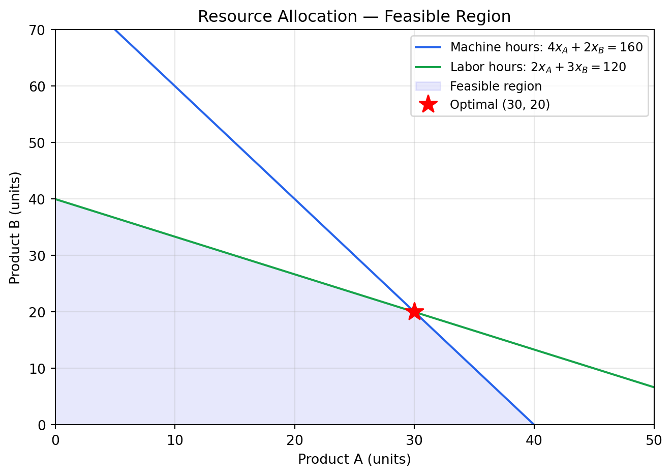
### Problem Statement: Resource Allocation
A small manufacturer produces two products — **Product A** and **Product B** — on
shared equipment. Each week the factory has:
- **160 hours** of machine time available
- **120 hours** of labor available
Resource requirements and profit margins:
| | Machine Hours | Labor Hours | Profit per Unit |
|---|---|---|---|
| Product A | 4 | 2 | $40 |
| Product B | 2 | 3 | $30 |
**Question:** How many units of each product should the factory produce each week to
maximize profit?
### Mathematical Formulation
Let $x_A$ = units of Product A produced per week, $x_B$ = units of Product B.
**Objective:**
$$\text{Maximize} \quad Z = 40x_A + 30x_B$$
**Subject to:**
$$4x_A + 2x_B \leq 160 \quad \text{(machine hours)}$$
$$2x_A + 3x_B \leq 120 \quad \text{(labor hours)}$$
$$x_A, x_B \geq 0 \quad \text{(non-negativity)}$$
### Python Implementation
```{python}
#| label: first-lp
#| fig-cap: "Feasible region and optimal solution for the resource allocation problem"
import pulp
import numpy as np
import matplotlib.pyplot as plt
import matplotlib.patches as mpatches

# --- Model ---
model = pulp.LpProblem("Resource_Allocation", pulp.LpMaximize)

x_a = pulp.LpVariable("Product_A", lowBound=0)
x_b = pulp.LpVariable("Product_B", lowBound=0)

# Objective
model += 40 * x_a + 30 * x_b, "Total_Profit"

# Constraints
model += 4 * x_a + 2 * x_b <= 160, "Machine_Hours"
model += 2 * x_a + 3 * x_b <= 120, "Labor_Hours"

# Solve
model.solve(pulp.PULP_CBC_CMD(msg=0))

x_a_opt = pulp.value(x_a)
x_b_opt = pulp.value(x_b)
profit   = pulp.value(model.objective)

print(f"Status       : {pulp.LpStatus[model.status]}")
print(f"Product A    : {x_a_opt:.1f} units")
print(f"Product B    : {x_b_opt:.1f} units")
print(f"Total Profit : ${profit:,.2f}")

# --- Visualization ---
fig, ax = plt.subplots(figsize=(7, 5))

x = np.linspace(0, 50, 400)

machine = (160 - 4 * x) / 2
labor   = (120 - 2 * x) / 3

ax.plot(x, machine, label="Machine hours: $4x_A + 2x_B = 160$", color="#2563eb")
ax.plot(x, labor,   label="Labor hours: $2x_A + 3x_B = 120$",   color="#16a34a")

# Feasible region vertices
vertices = np.array([[0, 0], [40, 0], [x_a_opt, x_b_opt], [0, 40]])
ax.fill(vertices[:, 0], vertices[:, 1], alpha=0.15, color="#6366f1", label="Feasible region")

ax.plot(x_a_opt, x_b_opt, "r*", markersize=14, label=f"Optimal ({x_a_opt:.0f}, {x_b_opt:.0f})")

ax.set_xlim(0, 50)
ax.set_ylim(0, 70)
ax.set_xlabel("Product A (units)")
ax.set_ylabel("Product B (units)")
ax.set_title("Resource Allocation — Feasible Region")
ax.legend(loc="upper right", fontsize=9)
ax.grid(True, alpha=0.3)
plt.tight_layout()
plt.show()
```
### Interpreting the Solution
The solver finds the optimal corner of the feasible region — the point where both
constraints bind simultaneously. Producing **24 units of Product A** and **24 units
of Product B** yields the maximum weekly profit of **$1,680**.
This result is not obvious from intuition. Product A has a higher profit margin ($40
vs $30), but it also consumes twice the machine hours. The optimal mix balances these
trade-offs mathematically, something that becomes impossible to do reliably as problems
grow to hundreds or thousands of variables.
---
## The OR-ML Workflow {#sec-workflow}
This book follows a consistent workflow for every problem class:
Problem Definition
↓
Data Collection & Exploration ← ML territory
↓
Model Formulation ← OR territory
↓
Algorithm Selection & Solving ← OR + ML
↓
Solution Validation
↓
Interpretation & Implementation
This workflow is not linear. Often, insights from data exploration will reshape the problem definition. Algorithm performance may lead to reformulating the model. The key is to iterate between these stages, using both OR and ML tools as needed to arrive at the best possible decision.
In practice these stages are iterative, not linear. A model that cannot be solved
efficiently sends you back to reformulation. A solution that makes no operational
sense sends you back to problem definition. The workflow is a compass, not a script.
---
## What Comes Next {#sec-next}
The remaining chapters in **Foundations** build the classical OR toolkit:
- **Linear Programming** — the geometry and algebra of continuous optimization,
the Simplex Method, duality, and sensitivity analysis
- **Integer Programming** — adding integrality constraints, branch-and-bound,
and combinatorial problems
- **Network Optimization** — shortest paths, minimum spanning trees, max flow,
and the transportation problem
Each chapter follows the same structure: theory, mathematical formulation, Python
implementation, and real-world case study. By the end of Foundations, you will have
the tools to formulate and solve a broad class of deterministic optimization problems —
and the intuition to know when those tools are and are not appropriate.
---
## Chapter Summary {#sec-summary}
- Operations Research applies mathematical modeling and optimization to improve decisions
under resource constraints
- Machine Learning discovers patterns in data to make predictions and automate decisions
- The two fields are converging: ML predicts, OR optimizes — together they form
prescriptive analytics
- Python provides a unified environment for both through `PuLP`, `scipy`, `scikit-learn`,
and related libraries
- Every OR problem has the same structure: decision variables, objective function,
constraints, and parameters
- The first LP example demonstrated formulation, implementation, solution, and
interpretation — the pattern this book follows throughout