---
title: "Probability and Statistics Foundations for OR and ML"
subtitle: "Chapter 2 – Part I: Foundations"
author: "Troy Altus"
date: "2026-04-14"
number-sections: true
number-depth: 3
---
## Why Probability and Statistics Matter {#sec-why-prob}
Linear algebra gives us the language of structure. Probability gives us the language
of **uncertainty** — and uncertainty is everywhere in real decisions.
Demand fluctuates. Travel times vary. Equipment fails without warning. Customers
behave unpredictably. Any model that ignores this variability will produce plans that
look optimal on paper but fail in practice.
In **Operations Research**, probability and statistics underpin:
- Stochastic programming — optimising over uncertain parameters
- Simulation — sampling system behaviour to evaluate decisions
- Queueing theory — modelling service systems under random arrivals
- Risk analysis — quantifying downside exposure in financial and operational models
In **Machine Learning**, they provide:
- The theoretical basis for model training (maximum likelihood, Bayesian inference)
- Tools for measuring and comparing model performance
- The language of uncertainty quantification (confidence intervals, prediction intervals)
- The foundation for probabilistic models (Naive Bayes, Gaussian processes, VAEs)
| Concept | OR Role | ML Role |
|---|---|---|
| Random variables | Uncertain demand, cost, time | Features, labels, noise |
| Distributions | Modelling variability | Likelihood functions, priors |
| Expectation | Expected cost/profit | Loss function minimisation |
| Variance | Risk quantification | Model variance (bias-variance tradeoff) |
| CLT | Justifying normal approximations in simulation | Generalisation bounds |
| Hypothesis testing | A/B testing operational changes | Model comparison, feature selection |
---
## Random Variables and Distributions {#sec-rv}
A **random variable** $X$ is a quantity whose value is determined by a random
experiment. It maps outcomes of a probability space to real numbers.
- **Discrete** random variables take a countable set of values (number of arrivals,
defects per batch, customers in a queue).
- **Continuous** random variables take values over an interval (service time, demand,
temperature).
### Probability Mass and Density Functions
For a **discrete** random variable, the **probability mass function (PMF)**
$p(x) = P(X = x)$ assigns probability to each outcome.
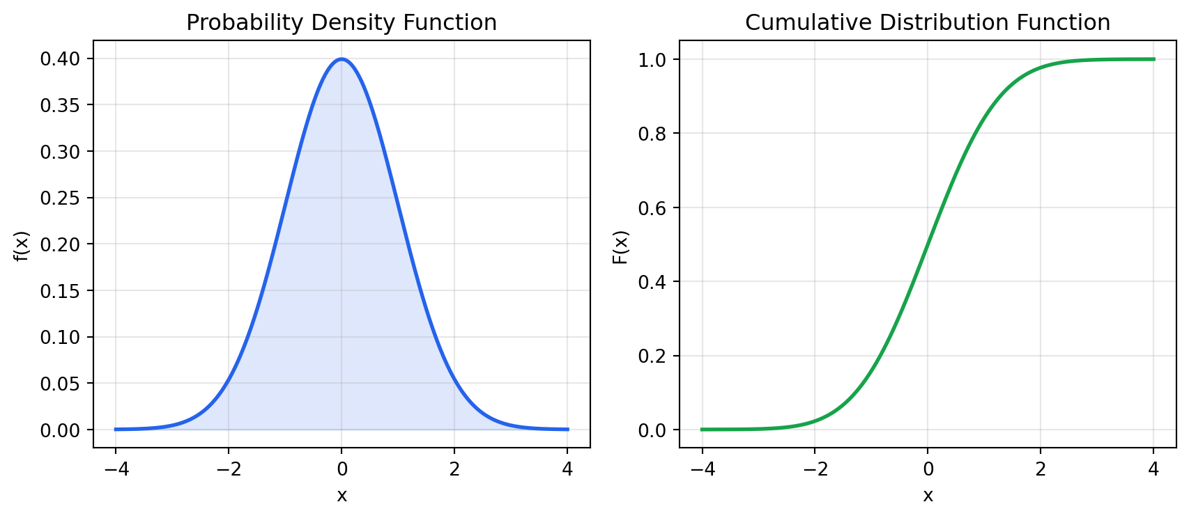
For a **continuous** random variable, the **probability density function (PDF)**
$f(x)$ satisfies:
$$P(a \leq X \leq b) = \int_a^b f(x)\, dx$$
No single point has positive probability — only intervals do.
The **cumulative distribution function (CDF)** works for both:
$$F(x) = P(X \leq x)$$
```{python}
#| label: fig-pdf-cdf
#| fig-cap: "PDF and CDF of the standard normal distribution"
import numpy as np
import matplotlib.pyplot as plt
from scipy import stats

x = np.linspace(-4, 4, 400)
dist = stats.norm(loc=0, scale=1)

fig, (ax1, ax2) = plt.subplots(1, 2, figsize=(9, 4))

ax1.plot(x, dist.pdf(x), color="#2563eb", lw=2)
ax1.fill_between(x, dist.pdf(x), alpha=0.15, color="#2563eb")
ax1.set_title("Probability Density Function")
ax1.set_xlabel("x")
ax1.set_ylabel("f(x)")
ax1.grid(True, alpha=0.3)

ax2.plot(x, dist.cdf(x), color="#16a34a", lw=2)
ax2.set_title("Cumulative Distribution Function")
ax2.set_xlabel("x")
ax2.set_ylabel("F(x)")
ax2.grid(True, alpha=0.3)

plt.tight_layout()
plt.show()
```
---
## Expectation, Variance, and Moments {#sec-moments}
### Expectation
The **expected value** (mean) of $X$ is its probability-weighted average:
$$\mathbb{E}[X] = \sum_x x \cdot p(x) \quad \text{(discrete)}$$
$$\mathbb{E}[X] = \int_{-\infty}^{\infty} x \cdot f(x)\, dx \quad \text{(continuous)}$$
Key properties:
- **Linearity:** $\mathbb{E}[aX + b] = a\mathbb{E}[X] + b$
- **Linearity of sums:** $\mathbb{E}[X + Y] = \mathbb{E}[X] + \mathbb{E}[Y]$ (always, regardless of dependence)
### Variance and Standard Deviation
**Variance** measures spread around the mean:
$$\text{Var}(X) = \mathbb{E}[(X - \mu)^2] = \mathbb{E}[X^2] - (\mathbb{E}[X])^2$$
**Standard deviation** $\sigma = \sqrt{\text{Var}(X)}$ has the same units as $X$.
For sums of **independent** random variables:
$$\text{Var}(X + Y) = \text{Var}(X) + \text{Var}(Y)$$
### Covariance and Correlation
**Covariance** measures linear association between two variables:
$$\text{Cov}(X, Y) = \mathbb{E}[(X - \mu_X)(Y - \mu_Y)]$$
**Pearson correlation** normalises to $[-1, 1]$:
$$\rho_{XY} = \frac{\text{Cov}(X, Y)}{\sigma_X \sigma_Y}$$
$\rho = 1$ means perfect positive linear relationship; $\rho = 0$ means no linear
relationship (but not necessarily independence).
```{python}
#| label: moments-demo
import numpy as np
from scipy import stats

np.random.seed(42)
demand = np.random.normal(loc=200, scale=30, size=10_000)

print(f"Mean     : {demand.mean():.2f}")
print(f"Variance : {demand.var():.2f}")
print(f"Std dev  : {demand.std():.2f}")
print(f"Skewness : {stats.skew(demand):.4f}")
print(f"Kurtosis : {stats.kurtosis(demand):.4f}")

# P(demand > 250)
prob_exceed = 1 - stats.norm.cdf(250, loc=200, scale=30)
print(f"\nP(demand > 250) = {prob_exceed:.4f}")
```
---
## Key Distributions {#sec-distributions}
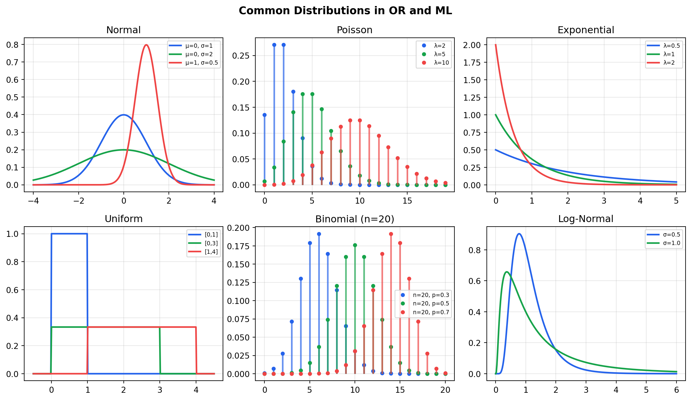
### Normal Distribution
$$X \sim \mathcal{N}(\mu, \sigma^2) \quad f(x) = \frac{1}{\sigma\sqrt{2\pi}} e^{-\frac{(x-\mu)^2}{2\sigma^2}}$$
**OR use:** Demand forecasting, machine processing times, measurement error.
**ML use:** Weight initialisation, noise modelling, Gaussian likelihoods.
The standard normal $Z \sim \mathcal{N}(0, 1)$ arises from standardising: $Z = (X - \mu)/\sigma$.
### Poisson Distribution
$$X \sim \text{Poisson}(\lambda) \quad P(X = k) = \frac{e^{-\lambda} \lambda^k}{k!}$$
Models the number of events in a fixed time interval, given a constant average rate
$\lambda$. Memoryless between events.
**OR use:** Customer arrivals per hour, orders per day, machine failures per week.
### Exponential Distribution
$$X \sim \text{Exp}(\lambda) \quad f(x) = \lambda e^{-\lambda x}, \quad x \geq 0$$
Models the *time between* Poisson-process events. Mean = $1/\lambda$.
**Key property — memorylessness:** $P(X > s + t \mid X > s) = P(X > t)$.
The remaining service time has the same distribution regardless of how long service
has already taken. This property makes it analytically tractable in queueing models.
**OR use:** Inter-arrival times, service times in $M/M/1$ queues.
### Uniform Distribution
$$X \sim \text{Uniform}(a, b) \quad f(x) = \frac{1}{b-a}, \quad x \in [a, b]$$
Every value in $[a, b]$ is equally likely. Mean $= (a+b)/2$, Var $= (b-a)^2/12$.
**OR use:** Initial bounds when no better information is available; simulation inputs.
### Bernoulli and Binomial
$$X \sim \text{Bernoulli}(p) \quad P(X=1) = p, \quad P(X=0) = 1-p$$
$$Y \sim \text{Binomial}(n, p) \quad P(Y=k) = \binom{n}{k} p^k (1-p)^{n-k}$$
$Y$ counts successes in $n$ independent Bernoulli trials.
**OR use:** Binary outcomes (on-time / late, defective / good), capacity thresholds.
**ML use:** Classification likelihoods, logistic regression.
```{python}
#| label: fig-distributions
#| fig-cap: "Key distributions used in OR and ML"
import numpy as np
import matplotlib.pyplot as plt
from scipy import stats

fig, axes = plt.subplots(2, 3, figsize=(12, 7))
axes = axes.flatten()

# Normal
x = np.linspace(-4, 4, 300)
for mu, sig, col in [(0, 1, "#2563eb"), (0, 2, "#16a34a"), (1, 0.5, "#ef4444")]:
    axes[0].plot(x, stats.norm.pdf(x, mu, sig), lw=2, color=col,
                 label=f"μ={mu}, σ={sig}")
axes[0].set_title("Normal"); axes[0].legend(fontsize=7); axes[0].grid(alpha=0.3)

# Poisson
k = np.arange(0, 20)
for lam, col in [(2, "#2563eb"), (5, "#16a34a"), (10, "#ef4444")]:
    pmf = stats.poisson.pmf(k, lam)
    axes[1].vlines(k, 0, pmf, color=col, lw=2, alpha=0.7)
    axes[1].plot(k, pmf, "o", color=col, ms=4, label=f"λ={lam}")
axes[1].set_title("Poisson"); axes[1].legend(fontsize=7); axes[1].grid(alpha=0.3)

# Exponential
x = np.linspace(0, 5, 300)
for lam, col in [(0.5, "#2563eb"), (1, "#16a34a"), (2, "#ef4444")]:
    axes[2].plot(x, stats.expon.pdf(x, scale=1/lam), lw=2, color=col,
                 label=f"λ={lam}")
axes[2].set_title("Exponential"); axes[2].legend(fontsize=7); axes[2].grid(alpha=0.3)

# Uniform
x = np.linspace(-0.5, 4.5, 300)
for a, b, col in [(0, 1, "#2563eb"), (0, 3, "#16a34a"), (1, 4, "#ef4444")]:
    axes[3].plot(x, stats.uniform.pdf(x, a, b-a), lw=2, color=col,
                 label=f"[{a},{b}]")
axes[3].set_title("Uniform"); axes[3].legend(fontsize=7); axes[3].grid(alpha=0.3)

# Binomial
k = np.arange(0, 21)
for n, p, col in [(20, 0.3, "#2563eb"), (20, 0.5, "#16a34a"), (20, 0.7, "#ef4444")]:
    pmf = stats.binom.pmf(k, n, p)
    axes[4].vlines(k, 0, pmf, color=col, lw=2, alpha=0.7)
    axes[4].plot(k, pmf, "o", color=col, ms=4, label=f"n=20, p={p}")
axes[4].set_title("Binomial (n=20)"); axes[4].legend(fontsize=7); axes[4].grid(alpha=0.3)

# Log-normal (common in finance, service times)
x = np.linspace(0, 6, 300)
for s, col in [(0.5, "#2563eb"), (1.0, "#16a34a")]:
    axes[5].plot(x, stats.lognorm.pdf(x, s), lw=2, color=col, label=f"σ={s}")
axes[5].set_title("Log-Normal"); axes[5].legend(fontsize=7); axes[5].grid(alpha=0.3)

plt.suptitle("Common Distributions in OR and ML", fontsize=13, fontweight="bold")
plt.tight_layout()
plt.show()
```
---
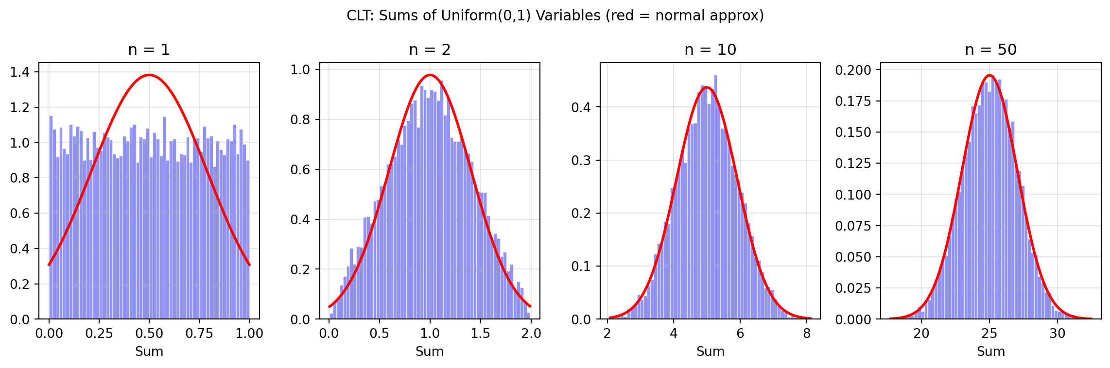
## The Central Limit Theorem {#sec-clt}
The **Central Limit Theorem (CLT)** is the most important result in applied statistics:
> **If $X_1, X_2, \ldots, X_n$ are i.i.d. random variables with mean $\mu$ and
> variance $\sigma^2$, then the sample mean $\bar{X}_n = \frac{1}{n}\sum X_i$
> converges in distribution to $\mathcal{N}(\mu, \sigma^2/n)$ as $n \to \infty$.**
In practice this means that sums and averages of many independent random variables
are approximately normally distributed — regardless of the underlying distribution.
**Why this matters in OR:**
- Total demand across many customers is approximately normal even if individual
orders are Poisson or uniform
- Average service time over many jobs converges to a normal distribution
- Simulation output means are approximately normal, enabling confidence intervals
**Why this matters in ML:**
- Justifies normal approximations to posterior distributions
- Underlies parametric confidence intervals for model metrics
- Central to bootstrap and permutation testing
```{python}
#| label: fig-clt
#| fig-cap: "CLT in action: sums of uniform random variables converge to normal"
import numpy as np
import matplotlib.pyplot as plt
from scipy import stats

np.random.seed(0)
N = 10_000

fig, axes = plt.subplots(1, 4, figsize=(12, 4))
for ax, n in zip(axes, [1, 2, 10, 50]):
    sample_means = np.random.uniform(0, 1, size=(N, n)).sum(axis=1)
    ax.hist(sample_means, bins=60, density=True, color="#6366f1", alpha=0.7,
            edgecolor="white", lw=0.3)
    # Overlay normal approximation
    mu_n  = n * 0.5
    sig_n = np.sqrt(n * (1/12))
    x = np.linspace(sample_means.min(), sample_means.max(), 300)
    ax.plot(x, stats.norm.pdf(x, mu_n, sig_n), "r-", lw=2)
    ax.set_title(f"n = {n}")
    ax.set_xlabel("Sum")
    ax.grid(True, alpha=0.3)

plt.suptitle("CLT: Sums of Uniform(0,1) Variables (red = normal approx)",
             fontsize=11)
plt.tight_layout()
plt.show()
```
---
## Estimation and Confidence Intervals {#sec-estimation}
### Point Estimation
A **point estimator** uses sample data to estimate a population parameter.
The **sample mean** $\bar{X} = \frac{1}{n}\sum_{i=1}^n X_i$ estimates $\mu$.
The **sample variance** $s^2 = \frac{1}{n-1}\sum_{i=1}^n (X_i - \bar{X})^2$ estimates $\sigma^2$.
A good estimator is:
- **Unbiased**: $\mathbb{E}[\hat{\theta}] = \theta$
- **Consistent**: $\hat{\theta} \to \theta$ as $n \to \infty$
- **Efficient**: minimum variance among unbiased estimators
### Confidence Intervals
A **95% confidence interval** is a procedure that, if repeated many times, would
contain the true parameter in 95% of repetitions. It is *not* a probability statement
about the specific interval computed from your sample.
For a sample mean with unknown $\sigma$ (the common case):
$$\bar{X} \pm t_{\alpha/2,\, n-1} \cdot \frac{s}{\sqrt{n}}$$
where $t_{\alpha/2,\, n-1}$ is the critical value from the $t$-distribution.
```{python}
#| label: confidence-intervals
import numpy as np
from scipy import stats

np.random.seed(7)

# Simulate 30 days of observed demand
demand_sample = np.random.normal(loc=200, scale=30, size=30)

n    = len(demand_sample)
mean = demand_sample.mean()
se   = demand_sample.std(ddof=1) / np.sqrt(n)

ci_90 = stats.t.interval(0.90, df=n-1, loc=mean, scale=se)
ci_95 = stats.t.interval(0.95, df=n-1, loc=mean, scale=se)
ci_99 = stats.t.interval(0.99, df=n-1, loc=mean, scale=se)

print(f"Sample mean   : {mean:.2f}")
print(f"Std error     : {se:.2f}")
print(f"90% CI        : ({ci_90[0]:.2f}, {ci_90[1]:.2f})")
print(f"95% CI        : ({ci_95[0]:.2f}, {ci_95[1]:.2f})")
print(f"99% CI        : ({ci_99[0]:.2f}, {ci_99[1]:.2f})")
```
Wider confidence intervals reflect greater uncertainty — either from more variability
($\sigma$) or less data ($n$). In OR, confidence intervals on simulation output
determine how many replications are needed to achieve a target precision.
---
## Hypothesis Testing {#sec-hypothesis-testing}
Hypothesis testing provides a formal framework for making decisions based on data.
### The Framework
1. **Null hypothesis $H_0$**: the status quo or baseline claim (e.g., "the new routing
policy does not reduce delivery time")
2. **Alternative hypothesis $H_1$**: what we want to detect (e.g., "the new policy
reduces delivery time")
3. **Test statistic**: a function of the data that measures evidence against $H_0$
4. **p-value**: probability of observing a test statistic at least as extreme as the
one computed, *if $H_0$ is true*
5. **Decision**: reject $H_0$ if $p < \alpha$ (significance level, typically 0.05)
A **Type I error** (false positive) rejects a true $H_0$; its rate is $\alpha$.
A **Type II error** (false negative) fails to reject a false $H_0$; its rate is $\beta$.
**Statistical power** = $1 - \beta$ = probability of correctly detecting a real effect.
### One-Sample t-Test
```{python}
#| label: t-test
import numpy as np
from scipy import stats

np.random.seed(3)

# Delivery times before and after a routing policy change
before = np.random.normal(loc=48, scale=8, size=50)  # hours
after  = np.random.normal(loc=44, scale=8, size=50)

t_stat, p_value = stats.ttest_ind(before, after, alternative="greater")

print(f"Mean before : {before.mean():.2f} hrs")
print(f"Mean after  : {after.mean():.2f} hrs")
print(f"t-statistic : {t_stat:.4f}")
print(f"p-value     : {p_value:.4f}")

alpha = 0.05
if p_value < alpha:
    print(f"\nReject H₀ at α={alpha}: new policy significantly reduces delivery time.")
else:
    print(f"\nFail to reject H₀ at α={alpha}: insufficient evidence.")
```
### Common Tests
| Test | When to Use |
|---|---|
| One-sample $t$ | Compare sample mean to a known value |
| Two-sample $t$ | Compare means of two independent groups |
| Paired $t$ | Compare means of matched pairs (before/after) |
| Chi-squared | Test independence of categorical variables |
| ANOVA | Compare means across three or more groups |
| Mann-Whitney U | Non-parametric alternative to two-sample $t$ |
| Kolmogorov-Smirnov | Test whether data follows a specified distribution |
---
## Bayesian vs. Frequentist Reasoning {#sec-bayes}
Two schools of thought underpin statistical inference in OR and ML:
**Frequentist** statistics treats probability as long-run frequency. Parameters are
fixed but unknown; only data is random. Inference is based on what would happen if the
experiment were repeated many times.
**Bayesian** statistics treats probability as a degree of belief. Parameters are
themselves random variables with prior distributions that are updated as data arrives.
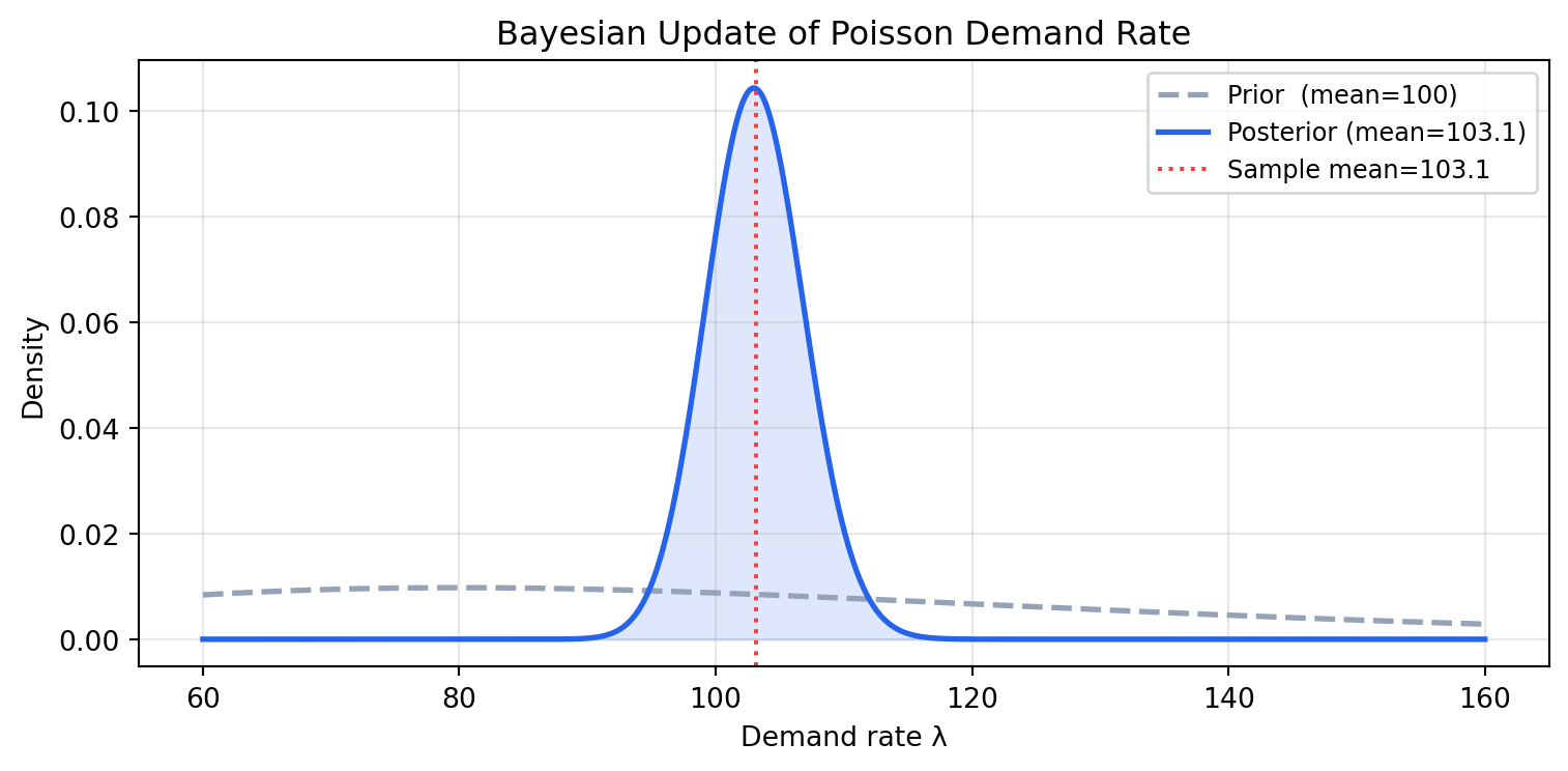
### Bayes' Theorem
$$P(\theta \mid \text{data}) = \frac{P(\text{data} \mid \theta) \cdot P(\theta)}{P(\text{data})}$$
- $P(\theta)$ — **prior**: belief about $\theta$ before seeing data
- $P(\text{data} \mid \theta)$ — **likelihood**: probability of the data given $\theta$
- $P(\theta \mid \text{data})$ — **posterior**: updated belief after seeing data
The posterior becomes the prior for the next update — Bayesian inference is sequential
and coherent.
```{python}
#| label: fig-bayes-update
#| fig-cap: "Bayesian updating: prior belief about demand rate updated with observed data"
import numpy as np
import matplotlib.pyplot as plt
from scipy import stats

# Estimating daily demand rate λ (Poisson)
# Prior: Gamma(alpha, beta) is conjugate prior for Poisson rate
# Posterior after observing n days with total demand S: Gamma(alpha + S, beta + n)

alpha_prior, beta_prior = 5, 0.05   # prior mean = alpha/beta = 100

observations = [95, 112, 88, 103, 117, 99, 108]   # 7 days of demand
n  = len(observations)
S  = sum(observations)

alpha_post = alpha_prior + S
beta_post  = beta_prior  + n

lam = np.linspace(60, 160, 500)
prior     = stats.gamma.pdf(lam, a=alpha_prior, scale=1/beta_prior)
posterior = stats.gamma.pdf(lam, a=alpha_post,  scale=1/beta_post)

fig, ax = plt.subplots(figsize=(8, 4))
ax.plot(lam, prior,     "--", color="#94a3b8", lw=2, label=f"Prior  (mean={alpha_prior/beta_prior:.0f})")
ax.plot(lam, posterior, "-",  color="#2563eb", lw=2,
        label=f"Posterior (mean={alpha_post/beta_post:.1f})")
ax.axvline(S/n, color="#ef4444", lw=1.5, linestyle=":", label=f"Sample mean={S/n:.1f}")
ax.fill_between(lam, posterior, alpha=0.15, color="#2563eb")
ax.set_xlabel("Demand rate λ")
ax.set_ylabel("Density")
ax.set_title("Bayesian Update of Poisson Demand Rate")
ax.legend(fontsize=9)
ax.grid(True, alpha=0.3)
plt.tight_layout()
plt.show()
```
The posterior is a compromise between the prior belief and the data. With more data,
the posterior concentrates around the true value and the prior's influence fades.
**In OR**, Bayesian methods appear in:
- Inventory models with uncertain demand (updating demand distribution as orders arrive)
- Predictive maintenance (updating failure rate estimates as machines age)
- Stochastic programming with distributional ambiguity
**In ML**, they appear in:
- Bayesian neural networks (weight distributions instead of point estimates)
- Gaussian processes (prior over functions)
- Hyperparameter optimisation (Bayesian optimisation)
---
## Monte Carlo Simulation {#sec-monte-carlo}
**Monte Carlo simulation** estimates quantities that are difficult to compute
analytically by sampling from probability distributions and averaging the results.
The core idea: if $Y = g(X_1, \ldots, X_n)$ and the $X_i$ are random with known
distributions, then:
$$\mathbb{E}[Y] \approx \frac{1}{N} \sum_{k=1}^N g(X_1^{(k)}, \ldots, X_n^{(k)})$$
By the CLT, this estimator is approximately normally distributed with standard error
$\sigma_Y / \sqrt{N}$ — halving the error requires quadrupling the sample size.
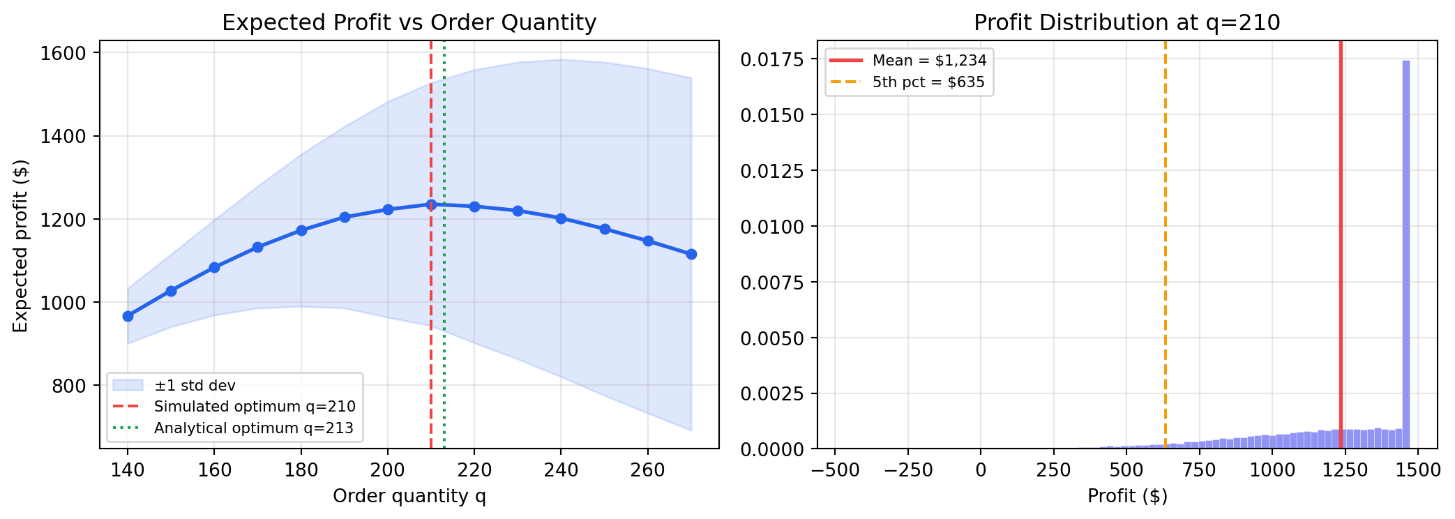
### Case Study: Newsvendor Problem
A retailer must order $q$ units of a perishable product *before* observing demand $D$.
Unsold units are wasted (cost $c_u$ per unit); unmet demand is lost (cost $c_o$ per unit).
**Optimal order quantity** (known analytically):
$$q^* = F^{-1}\!\left(\frac{c_u - c}{c_u + c_o - c}\right)$$
where $c$ is unit cost. Monte Carlo lets us estimate profit distributions for any $q$.
```{python}
#| label: fig-newsvendor
#| fig-cap: "Newsvendor profit distribution: Monte Carlo simulation over order quantities"
import numpy as np
import matplotlib.pyplot as plt
from scipy import stats

np.random.seed(42)

# Parameters
unit_cost      = 5    # cost per unit ordered
unit_price     = 12   # revenue per unit sold
salvage_value  = 1    # value of unsold units
N              = 50_000

# Demand: normally distributed
mu_demand, sig_demand = 200, 40

def simulate_profit(q, n=N):
    demand  = np.random.normal(mu_demand, sig_demand, n).clip(0)
    sold    = np.minimum(q, demand)
    unsold  = np.maximum(q - demand, 0)
    revenue = sold * unit_price + unsold * salvage_value
    cost    = q * unit_cost
    return revenue - cost

order_quantities = range(140, 280, 10)
mean_profits = []
std_profits  = []

for q in order_quantities:
    profits = simulate_profit(q)
    mean_profits.append(profits.mean())
    std_profits.append(profits.std())

mean_profits = np.array(mean_profits)
std_profits  = np.array(std_profits)
qs = np.array(list(order_quantities))

best_q = qs[mean_profits.argmax()]

# Analytical optimum (critical ratio)
cr = (unit_price - unit_cost) / (unit_price - salvage_value)
q_star = int(stats.norm.ppf(cr, loc=mu_demand, scale=sig_demand))

fig, (ax1, ax2) = plt.subplots(1, 2, figsize=(11, 4))

ax1.plot(qs, mean_profits, color="#2563eb", lw=2, marker="o", ms=5)
ax1.fill_between(qs, mean_profits - std_profits, mean_profits + std_profits,
                 alpha=0.15, color="#2563eb", label="±1 std dev")
ax1.axvline(best_q,  color="#ef4444", lw=1.5, linestyle="--",
            label=f"Simulated optimum q={best_q}")
ax1.axvline(q_star, color="#16a34a", lw=1.5, linestyle=":",
            label=f"Analytical optimum q={q_star}")
ax1.set_xlabel("Order quantity q")
ax1.set_ylabel("Expected profit ($)")
ax1.set_title("Expected Profit vs Order Quantity")
ax1.legend(fontsize=8)
ax1.grid(True, alpha=0.3)

# Profit distribution at optimal q
profits_opt = simulate_profit(best_q)
ax2.hist(profits_opt, bins=80, density=True, color="#6366f1", alpha=0.7,
         edgecolor="white", lw=0.2)
ax2.axvline(profits_opt.mean(), color="#ef4444", lw=2,
            label=f"Mean = ${profits_opt.mean():,.0f}")
ax2.axvline(np.percentile(profits_opt, 5), color="#f59e0b", lw=1.5,
            linestyle="--", label=f"5th pct = ${np.percentile(profits_opt,5):,.0f}")
ax2.set_xlabel("Profit ($)")
ax2.set_title(f"Profit Distribution at q={best_q}")
ax2.legend(fontsize=8)
ax2.grid(True, alpha=0.3)

plt.tight_layout()
plt.show()

print(f"Simulated optimal order : {best_q} units")
print(f"Analytical optimal order: {q_star} units")
print(f"Expected profit at q={best_q}: ${simulate_profit(best_q).mean():,.2f}")
print(f"5th percentile (downside) : ${np.percentile(simulate_profit(best_q), 5):,.2f}")
```
Monte Carlo confirms the analytical result and adds something the formula cannot
provide: the full profit *distribution*, including downside risk quantified by
percentiles. A risk-averse manager might choose $q < q^*$ to reduce variance even
at the cost of expected profit.
---
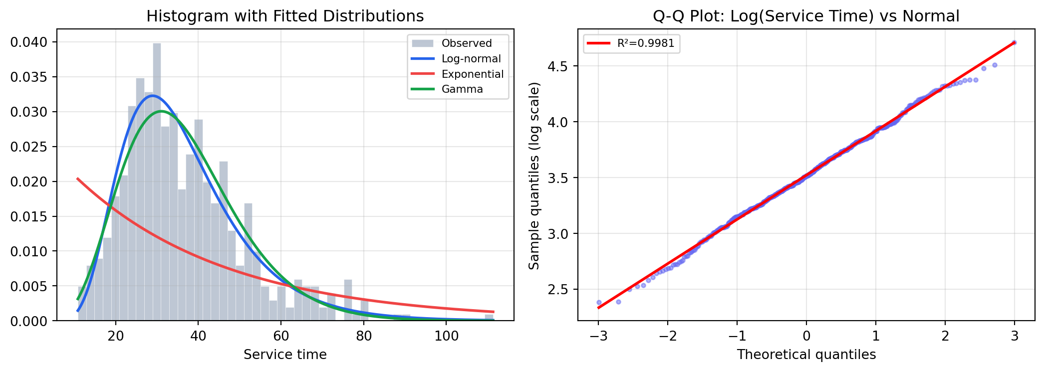
## Fitting Distributions to Data {#sec-fitting}
In practice, the demand or service-time distribution is unknown and must be estimated
from historical data. The standard approach:
1. **Visualise** — histogram, Q-Q plot
2. **Fit candidates** — maximum likelihood estimation (MLE)
3. **Test goodness of fit** — Kolmogorov-Smirnov or Chi-squared test
```{python}
#| label: fig-distribution-fitting
#| fig-cap: "Fitting a log-normal distribution to historical service times"
import numpy as np
import matplotlib.pyplot as plt
from scipy import stats

np.random.seed(1)
# Simulate historical service times (log-normal: right-skewed, positive-only)
true_mu, true_sigma = 3.5, 0.4
service_times = np.random.lognormal(mean=true_mu, sigma=true_sigma, size=500)

# Fit candidates
fit_lognorm = stats.lognorm.fit(service_times, floc=0)
fit_expon   = stats.expon.fit(service_times,   floc=0)
fit_gamma   = stats.gamma.fit(service_times,   floc=0)

# KS tests
ks_lognorm = stats.kstest(service_times, "lognorm", args=fit_lognorm)
ks_expon   = stats.kstest(service_times, "expon",   args=fit_expon)
ks_gamma   = stats.kstest(service_times, "gamma",   args=fit_gamma)

print("Goodness-of-fit (KS test):")
print(f"  Log-normal : KS={ks_lognorm.statistic:.4f}, p={ks_lognorm.pvalue:.4f}")
print(f"  Exponential: KS={ks_expon.statistic:.4f},   p={ks_expon.pvalue:.4f}")
print(f"  Gamma      : KS={ks_gamma.statistic:.4f},   p={ks_gamma.pvalue:.4f}")

fig, (ax1, ax2) = plt.subplots(1, 2, figsize=(11, 4))

x = np.linspace(service_times.min(), service_times.max(), 300)
ax1.hist(service_times, bins=50, density=True, color="#94a3b8",
         alpha=0.6, label="Observed", edgecolor="white", lw=0.3)
ax1.plot(x, stats.lognorm.pdf(x, *fit_lognorm), color="#2563eb", lw=2, label="Log-normal")
ax1.plot(x, stats.expon.pdf(x, *fit_expon),     color="#ef4444", lw=2, label="Exponential")
ax1.plot(x, stats.gamma.pdf(x, *fit_gamma),     color="#16a34a", lw=2, label="Gamma")
ax1.set_xlabel("Service time")
ax1.set_title("Histogram with Fitted Distributions")
ax1.legend(fontsize=8)
ax1.grid(True, alpha=0.3)

# Q-Q plot for best fit (log-normal)
(osm, osr), (slope, intercept, r) = stats.probplot(
    np.log(service_times), dist="norm"
)
ax2.plot(osm, osr, "o", color="#6366f1", ms=3, alpha=0.5)
ax2.plot(osm, slope * np.array(osm) + intercept, "r-", lw=2, label=f"R²={r**2:.4f}")
ax2.set_xlabel("Theoretical quantiles")
ax2.set_ylabel("Sample quantiles (log scale)")
ax2.set_title("Q-Q Plot: Log(Service Time) vs Normal")
ax2.legend(fontsize=8)
ax2.grid(True, alpha=0.3)

plt.tight_layout()
plt.show()
```
A high KS p-value means the data is consistent with the fitted distribution — we lack
evidence to reject it. A log-normal is appropriate when values are positive and
right-skewed (service times, income, firm sizes).
---
## Chapter Summary {#sec-prob-summary}
- **Random variables** model uncertain quantities; their distributions encode all
probabilistic information
- **Expectation** gives the probability-weighted average; **variance** measures spread;
**covariance** measures linear co-movement
- Key distributions for OR: Normal (symmetric continuous), Poisson (discrete counts),
Exponential (inter-arrival times), Uniform (bounded uncertainty), Binomial (binary trials)
- The **Central Limit Theorem** guarantees that sums and averages converge to normal
distributions — justifying normal approximations throughout simulation and inference
- **Confidence intervals** and **hypothesis tests** formalise decision-making from
sample data; t-tests, Chi-squared tests, and KS tests are the most common tools
- **Bayesian inference** updates prior beliefs with data via Bayes' theorem; conjugate
priors (Gamma-Poisson) yield analytical posteriors
- **Monte Carlo simulation** estimates expected values and full distributions for
analytically intractable problems — the newsvendor example shows how it combines
with optimisation to reveal both expected profit and downside risk
- **Distribution fitting** (MLE + KS test + Q-Q plot) is the standard workflow for
determining the right distributional assumption from historical data