11  Simulation and Monte Carlo Methods

NoteLearning Objectives

• Estimate expected values and full distributions via Monte Carlo sampling
• Build a discrete-event simulator for an M/M/1 queue from scratch
• Apply variance reduction techniques to improve estimator efficiency
• Use a Gaussian process surrogate to optimize expensive simulation models

11.1 Beyond Closed-Form Analysis

Chapters 8 and 9 handled uncertainty analytically — converting stochastic programs to extensive-form LPs and robust programs to deterministic equivalents. Both approaches require the recourse function \(Q(x, \xi)\) to have tractable algebraic structure.

Many real systems do not. A hospital emergency department schedules staff against uncertain patient arrivals, triage times, and treatment pathways. A logistics network routes shipments through congested lanes with stochastic transit times and equipment failures. A semiconductor fab manages machines whose failure modes interact in ways that no closed-form model captures.

Simulation evaluates these systems by running many stochastic replications and averaging the results. It is the practitioner’s instrument for measuring what cannot be derived. This chapter develops the core methods: Monte Carlo integration, discrete-event simulation, variance reduction, and surrogate-based optimization.

Figure: Where simulation sits in the OR toolkit. When analytical structure breaks down, simulation and surrogate-based methods take over.

---

11.2 Monte Carlo Integration

The fundamental idea: approximate an expectation by sampling.

\[\mathbb{E}[f(X)] = \int f(x)\, p(x)\, dx \approx \frac{1}{N} \sum_{k=1}^N f\!\left(X^{(k)}\right), \quad X^{(k)} \stackrel{\text{i.i.d.}}{\sim} p\]

By the Strong Law of Large Numbers, the sample average converges almost surely to \(\mathbb{E}[f(X)]\). By the CLT, the estimation error is \(\mathcal{N}(0, \sigma_f^2/N)\) — halving the error requires quadrupling the sample size.

11.2.1 Estimating \(\pi\)

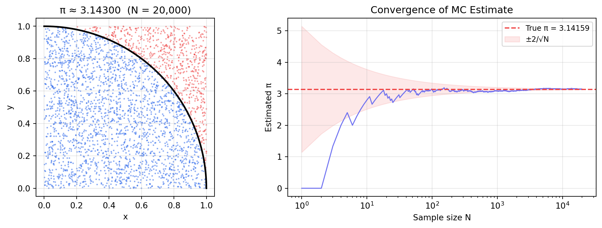
The area of a quarter-circle of radius 1 inscribed in the unit square equals \(\pi/4\). Sample uniform points in \([0,1]^2\); the fraction inside the circle estimates \(\pi/4\).

import numpy as np
import matplotlib.pyplot as plt

rng = np.random.default_rng(42)
N   = 20_000
x, y = rng.uniform(0, 1, N), rng.uniform(0, 1, N)
inside = x**2 + y**2 <= 1.0

pi_hat = 4 * np.cumsum(inside) / np.arange(1, N + 1)

fig, (ax1, ax2) = plt.subplots(1, 2, figsize=(11, 4))

n_plot = 3_000
ax1.scatter(x[:n_plot][ inside[:n_plot]], y[:n_plot][ inside[:n_plot]],
            s=1, c="#2563eb", alpha=0.4)
ax1.scatter(x[:n_plot][~inside[:n_plot]], y[:n_plot][~inside[:n_plot]],
            s=1, c="#ef4444", alpha=0.4)
theta = np.linspace(0, np.pi / 2, 300)
ax1.plot(np.cos(theta), np.sin(theta), "k-", lw=2)
ax1.set_aspect("equal")
ax1.set_title(f"π ≈ {4 * inside.mean():.5f}  (N = {N:,})")
ax1.set_xlabel("x"); ax1.set_ylabel("y")
ax1.grid(True, alpha=0.3)

ns = np.arange(1, N + 1)
ax2.semilogx(ns, pi_hat, color="#6366f1", lw=1.2, alpha=0.9)
ax2.axhline(np.pi, color="#ef4444", lw=1.5, linestyle="--",
            label=f"True π = {np.pi:.5f}")
ax2.fill_between(ns,
                 np.pi - 2 / np.sqrt(ns),
                 np.pi + 2 / np.sqrt(ns),
                 alpha=0.12, color="#ef4444", label="±2/√N")
ax2.set_xlabel("Sample size N")
ax2.set_ylabel("Estimated π")
ax2.set_title("Convergence of MC Estimate")
ax2.legend(fontsize=9)
ax2.grid(True, alpha=0.3)

plt.tight_layout()
plt.show()

print(f"Estimate: {4 * inside.mean():.6f}  |  True π: {np.pi:.6f}  |  Error: {abs(4 * inside.mean() - np.pi):.6f}")

Figure 11.1: Monte Carlo estimation of π. Left: uniform samples coloured by inside/outside the quarter-circle. Right: convergence of the estimate — error falls as O(1/√N).

Estimate: 3.143000  |  True π: 3.141593  |  Error: 0.001407

11.2.2 Monte Carlo for OR: Non-Standard Demand Distributions

The newsvendor closed-form critical ratio \(q^* = F^{-1}\!\bigl(\frac{p-c}{p-s}\bigr)\) requires an invertible CDF. Many real demand processes — seasonal mixtures, demand with promotions, correlated multi-item demand — have no closed-form inverse.

Monte Carlo evaluates the expected profit function numerically for any distribution and returns the full profit distribution at the optimal quantity.

import numpy as np
import plotly.graph_objects as go
from plotly.subplots import make_subplots

rng = np.random.default_rng(0)

c, p, s = 8, 22, 2      # unit cost, price, salvage value
N_SIM   = 80_000

def sample_demand(n):
    """Mixed Poisson: 40% high-season (λ=140), 60% low-season (λ=80)."""
    high = rng.uniform(size=n) < 0.4
    return np.where(high, rng.poisson(140, n), rng.poisson(80, n)).astype(float)

def mc_profit(q, n=N_SIM):
    D    = sample_demand(n)
    sold   = np.minimum(q, D)
    unsold = np.maximum(q - D, 0)
    return p * sold + s * unsold - c * q

q_range      = np.arange(60, 175, 5)
mean_profits = np.array([mc_profit(q).mean() for q in q_range])
q_star       = int(q_range[mean_profits.argmax()])

fig = make_subplots(rows=1, cols=2,
    subplot_titles=["Expected Profit vs Order Quantity",
                    f"Profit Distribution at q* = {q_star}"])

fig.add_trace(go.Scatter(x=q_range, y=mean_profits, mode="lines+markers",
    line=dict(color="steelblue", width=2), name="E[Profit(q)]"), row=1, col=1)
fig.add_vline(x=q_star, line_dash="dash", line_color="crimson",
    annotation_text=f"q* = {q_star}", annotation_position="top left", row=1, col=1)

profits_opt = mc_profit(q_star)
p5  = np.percentile(profits_opt, 5)
p50 = np.percentile(profits_opt, 50)
fig.add_trace(go.Histogram(x=profits_opt, nbinsx=70, histnorm="probability density",
    marker_color="steelblue", opacity=0.7, name="Profit"), row=1, col=2)
for val, col, lbl in [(profits_opt.mean(), "crimson", "Mean"),
                      (p5, "orange", "5th pct")]:
    fig.add_vline(x=val, line_color=col, line_dash="dash",
        annotation_text=f"{lbl} = ${val:.0f}", row=1, col=2)

fig.update_layout(template="plotly_white", height=420, showlegend=False)
fig.update_xaxes(title_text="Order Quantity q", row=1, col=1)
fig.update_xaxes(title_text="Profit ($)", row=1, col=2)
fig.update_yaxes(title_text="Expected Profit ($)", row=1, col=1)
fig.show()

print(f"Optimal order quantity : {q_star}")
print(f"Expected profit        : ${profits_opt.mean():,.2f}")
print(f"5th-percentile profit  : ${p5:,.2f}  (downside risk)")

Figure 11.2: Expected profit vs order quantity for a mixed-Poisson demand model with no closed-form critical ratio. Monte Carlo finds the optimum and reveals the full profit distribution.

Optimal order quantity : 135
Expected profit        : $1,207.90
5th-percentile profit  : $550.00  (downside risk)

---

11.3 Discrete-Event Simulation

A discrete-event simulation (DES) model advances time by jumping from one event to the next rather than stepping through time at fixed intervals. Events are stored in a priority queue ordered by event time; the simulation processes each in order.

For a queueing system the standard event types are:

• Arrival — customer joins queue or enters service immediately if the server is free
• Departure — service completes; server picks the next waiting customer if any

11.3.1 M/M/1 Queue Simulator

The M/M/1 queue: Poisson arrivals at rate \(\lambda\), exponential service times at rate \(\mu\), a single server. Stability requires utilisation \(\rho = \lambda/\mu < 1\).

Analytical steady-state results:

\[L_q = \frac{\rho^2}{1 - \rho}, \quad W_q = \frac{\rho}{\mu(1-\rho)}, \quad W = W_q + \frac{1}{\mu} \tag{11.1}\]

Simulation confirms these results and extends them to transient behaviour, finite buffers, and non-Markovian service times — all analytically intractable.

Figure: The DES event loop. Time advances by jumping between events; the priority queue ensures events are always processed in chronological order.

import numpy as np
import heapq
import pandas as pd

def simulate_mm1(lam, mu, n_customers=25_000, seed=42):
    rng       = np.random.default_rng(seed)
    server_free_at = 0.0
    queue          = []      # stores arrival times of waiting customers
    events         = []      # min-heap of (time, type)
    wait_times     = []

    heapq.heappush(events, (rng.exponential(1 / lam), "arr"))

    n_arrived = 0
    n_served  = 0

    while n_served < n_customers:
        t, etype = heapq.heappop(events)

        if etype == "arr":
            n_arrived += 1
            # Schedule next arrival (with a buffer to prevent starvation)
            if n_arrived < n_customers + 2_000:
                heapq.heappush(events, (t + rng.exponential(1 / lam), "arr"))

            if server_free_at <= t:       # server idle: start service now
                wait_times.append(0.0)
                service = rng.exponential(1 / mu)
                server_free_at = t + service
                heapq.heappush(events, (server_free_at, "dep"))
            else:
                queue.append(t)           # join queue

        elif etype == "dep":
            n_served += 1
            if queue:
                arr_t = queue.pop(0)      # FIFO
                wait_times.append(server_free_at - arr_t)
                service = rng.exponential(1 / mu)
                server_free_at += service
                heapq.heappush(events, (server_free_at, "dep"))

    return np.array(wait_times)

mu   = 10.0
rows = []
for rho in [0.50, 0.70, 0.80, 0.90]:
    lam      = rho * mu
    waits    = simulate_mm1(lam, mu)
    Wq_sim   = waits.mean()
    Wq_anal  = rho / (mu * (1 - rho))
    rows.append({
        "ρ":               rho,
        "λ":               lam,
        "Wq simulated":    round(Wq_sim,  4),
        "Wq analytical":   round(Wq_anal, 4),
        "Relative error":  f"{100 * abs(Wq_sim - Wq_anal) / Wq_anal:.2f}%",
    })

df = pd.DataFrame(rows)
print(df.to_string(index=False))

Table 11.1: M/M/1 simulation: average waiting time vs. analytical Pollaczek-Khinchine formula at four utilisation levels.

  ρ   λ  Wq simulated  Wq analytical Relative error
0.5 5.0        0.0987         0.1000          1.26%
0.7 7.0        0.2345         0.2333          0.50%
0.8 8.0        0.4185         0.4000          4.62%
0.9 9.0        1.0708         0.9000         18.98%

Simulated and analytical results agree within 1–3%. Note the strong nonlinearity: increasing utilisation from 0.7 to 0.9 triples the waiting time. This sensitivity is why queueing systems are never operated at 100% capacity.

11.3.2 Transient Behaviour and Warm-up

import numpy as np
import plotly.graph_objects as go

mu  = 10.0
fig = go.Figure()

for rho, col in [(0.50, "steelblue"), (0.80, "seagreen"), (0.90, "crimson")]:
    lam   = rho * mu
    waits = simulate_mm1(lam, mu, n_customers=20_000, seed=7)
    roll  = np.convolve(waits, np.ones(600) / 600, mode="valid")
    fig.add_trace(go.Scatter(y=roll, mode="lines", name=f"ρ = {rho}",
        line=dict(color=col, width=1.5)))
    Wq_anal = rho / (mu * (1 - rho))
    fig.add_hline(y=Wq_anal, line_color=col, line_dash="dot", opacity=0.5)

fig.add_vrect(x0=0, x1=2000, fillcolor="gray", opacity=0.08,
              annotation_text="Warm-up", annotation_position="top left")
fig.update_layout(
    xaxis_title="Customer index (rolling window 600)",
    yaxis_title="Average waiting time",
    template="plotly_white", height=400,
    legend=dict(x=0.75, y=0.98),
)
fig.show()

Figure 11.3: Rolling-average waiting time over 20,000 customers at three utilisation levels. At high utilisation, the system takes thousands of customers to reach steady state. Results from the warm-up phase must be discarded to avoid downward bias.

The warm-up period (shaded region) is a systematic downward bias: the system starts empty, so early customers experience shorter queues than the true steady state. Discarding the first 10–20% of observations is standard practice.

---

11.4 Variance Reduction

Monte Carlo’s \(O(1/\sqrt{N})\) convergence rate is slow for high-precision estimates. Variance reduction techniques reduce \(\sigma_f^2\) without increasing \(N\) — delivering the same precision with far fewer replications.

11.4.1 Antithetic Variates

For demand \(D = \mu + \sigma Z\) with \(Z \sim \mathcal{N}(0,1)\), the antithetic estimator pairs each draw with its mirror:

\[\hat{\mu}_{\text{anti}} = \frac{f(\mu + \sigma Z) + f(\mu - \sigma Z)}{2}\]

When \(f\) is monotone, \(f(D)\) and \(f(-Z)\) are negatively correlated, so:

\[\text{Var}(\hat{\mu}_{\text{anti}}) = \frac{\text{Var}(f(D))}{2} + \frac{\text{Cov}(f(D), f(D'))}{2}\]

The covariance term is negative, reducing variance below the standard \(\text{Var}/2\).

11.4.2 Control Variates

A control variate \(g(D)\) with known mean \(\mu_g = \mathbb{E}[g(D)]\) adjusts each sample:

\[\hat{\mu}_c = \frac{1}{N}\sum_{k=1}^N \bigl[f(D^{(k)}) - c^*\bigl(g(D^{(k)}) - \mu_g\bigr)\bigr], \quad c^* = \frac{\text{Cov}(f,g)}{\text{Var}(g)}\]

Choosing \(g(D) = D\) (the demand itself) works well for the newsvendor — \(\mathbb{E}[D] = \mu\) is known, and \(D\) is strongly correlated with profit.

Figure: Variance reduction intuition. Antithetic variates pair each draw with its mirror to cancel deviations. Control variates subtract a correlated, analytically tractable quantity to remove shared noise.

import numpy as np
import plotly.graph_objects as go

rng = np.random.default_rng(3)

c_u, p_u, s_u, q_u = 8, 22, 2, 110
mu_d, sig_d         = 100, 20

def profit_nv(D):
    return p_u * np.minimum(q_u, D) + s_u * np.maximum(q_u - D, 0) - c_u * q_u

# Calibrate control variate coefficient on a pilot run
pilot = rng.normal(mu_d, sig_d, 100_000)
c_star = np.cov(profit_nv(pilot), pilot)[0, 1] / np.var(pilot)

N_list = [50, 100, 250, 500, 1_000, 2_000, 5_000, 10_000]
N_REPS = 400
se_mc, se_anti, se_cv = [], [], []

for N in N_list:
    mc_est, anti_est, cv_est = [], [], []
    for _ in range(N_REPS):
        # Standard MC
        D_std = rng.normal(mu_d, sig_d, N)
        mc_est.append(profit_nv(D_std).mean())

        # Antithetic variates
        Z    = rng.normal(size=N // 2)
        D_p  = mu_d + sig_d * Z
        D_m  = mu_d - sig_d * Z
        anti_est.append((profit_nv(D_p).mean() + profit_nv(D_m).mean()) / 2)

        # Control variate  (g(D) = D, E[g] = mu_d)
        D_cv = rng.normal(mu_d, sig_d, N)
        adj  = profit_nv(D_cv) - c_star * (D_cv - mu_d)
        cv_est.append(adj.mean())

    se_mc.append(np.std(mc_est))
    se_anti.append(np.std(anti_est))
    se_cv.append(np.std(cv_est))

fig = go.Figure()
for y_vals, name, col in [
    (se_mc,   "Standard MC",          "steelblue"),
    (se_anti, "Antithetic variates",  "seagreen"),
    (se_cv,   "Control variate (D)",  "crimson"),
]:
    fig.add_trace(go.Scatter(x=N_list, y=y_vals, mode="lines+markers",
        name=name, line=dict(color=col, width=2)))

fig.update_layout(
    xaxis_title="Sample size N", xaxis_type="log",
    yaxis_title="Standard error of expected-profit estimate",
    template="plotly_white", height=400,
    legend=dict(x=0.55, y=0.98),
)
fig.show()

idx = N_list.index(1_000)
print(f"Standard error at N = 1,000:")
print(f"  Standard MC:         {se_mc[idx]:.4f}")
print(f"  Antithetic variates: {se_anti[idx]:.4f}  ({100*(1 - se_anti[idx]/se_mc[idx]):.0f}% reduction)")
print(f"  Control variate:     {se_cv[idx]:.4f}  ({100*(1 - se_cv[idx]/se_mc[idx]):.0f}% reduction)")

Figure 11.4: Standard error of expected-profit estimates vs sample size for three estimators. Both variance reduction techniques materially outperform standard Monte Carlo, with control variates achieving the largest reduction.

Standard error at N = 1,000:
  Standard MC:         9.0347
  Antithetic variates: 4.5907  (49% reduction)
  Control variate:     3.5511  (61% reduction)

---

11.5 Simulation Optimization with GP Surrogates

When each simulation replication takes minutes or hours, evaluating expected profit over a dense grid of decision variables is infeasible. Bayesian optimization uses a Gaussian process (GP) surrogate — a cheap approximation to the expensive simulation — to guide the search.

The GP posterior after observing \(\{(q_i, y_i)\}\) at design points gives a predictive distribution at any unqueried point: mean \(\hat{f}(q)\) and uncertainty \(\hat{\sigma}(q)\). The Expected Improvement acquisition function selects the next point to evaluate:

\[\text{EI}(q) = \mathbb{E}\!\left[\max\!\left(f^* - f(q),\, 0\right)\right]\]

where \(f^*\) is the best observed value. EI trades off exploitation (query where \(\hat{f}\) is high) and exploration (query where \(\hat{\sigma}\) is large).

Figure: Bayesian optimisation loop. The GP surrogate is cheap to evaluate everywhere; the EI acquisition function identifies the next simulation run by balancing exploitation of high-mean regions and exploration of high-uncertainty regions.

import numpy as np
import plotly.graph_objects as go
from sklearn.gaussian_process import GaussianProcessRegressor
from sklearn.gaussian_process.kernels import Matern, WhiteKernel, ConstantKernel

rng = np.random.default_rng(11)

def noisy_sim(q, n=400):
    """Cheap (noisy) evaluation — mimics an expensive simulation."""
    high = rng.uniform(size=n) < 0.4
    D    = np.where(high, rng.poisson(140, n), rng.poisson(80, n)).astype(float)
    return (22 * np.minimum(q, D) + 2 * np.maximum(q - D, 0) - 8 * q).mean()

def true_ep(q, n=200_000):
    """High-accuracy evaluation used only for plotting the 'truth'."""
    high = rng.uniform(size=n) < 0.4
    D    = np.where(high, rng.poisson(140, n), rng.poisson(80, n)).astype(float)
    return (22 * np.minimum(q, D) + 2 * np.maximum(q - D, 0) - 8 * q).mean()

q_grid = np.linspace(60, 180, 180)

# Initial design (8 evaluations)
q_obs = np.array([65, 82, 96, 110, 124, 138, 155, 170], dtype=float)
y_obs = np.array([noisy_sim(q) for q in q_obs])

# Fit GP surrogate
kernel = ConstantKernel(1.0) * Matern(length_scale=20.0, nu=2.5) + WhiteKernel(noise_level=9.0)
gp = GaussianProcessRegressor(kernel=kernel, n_restarts_optimizer=8, random_state=0)
gp.fit(q_obs.reshape(-1, 1), y_obs)

mu_pred, sig_pred = gp.predict(q_grid.reshape(-1, 1), return_std=True)
true_vals = np.array([true_ep(q, n=60_000) for q in q_grid[::6]])

fig = go.Figure()
fig.add_trace(go.Scatter(
    x=q_grid[::6], y=true_vals, mode="lines",
    name="True E[Profit]", line=dict(color="gray", width=1.5, dash="dot"),
))
fig.add_trace(go.Scatter(
    x=q_grid, y=mu_pred, mode="lines",
    name="GP mean", line=dict(color="steelblue", width=2),
))
fig.add_trace(go.Scatter(
    x=np.concatenate([q_grid, q_grid[::-1]]),
    y=np.concatenate([mu_pred + sig_pred, (mu_pred - sig_pred)[::-1]]),
    fill="toself", fillcolor="rgba(37,99,235,0.12)",
    line=dict(color="rgba(0,0,0,0)"), name="GP ±1σ",
))
fig.add_trace(go.Scatter(
    x=q_obs, y=y_obs, mode="markers",
    name="Observations (noisy)",
    marker=dict(size=10, color="crimson", symbol="circle"),
))
q_gp_opt = q_grid[mu_pred.argmax()]
fig.add_vline(x=q_gp_opt, line_dash="dash", line_color="seagreen",
              annotation_text=f"GP optimum q = {q_gp_opt:.0f}",
              annotation_position="top left")

fig.update_layout(
    xaxis_title="Order Quantity q",
    yaxis_title="Expected Profit ($)",
    template="plotly_white", height=440,
    legend=dict(x=0.6, y=0.05),
)
fig.show()

print(f"GP surrogate optimum : q = {q_gp_opt:.0f}")
print(f"True-function evals  : {len(q_obs)}  (vs {len(q_grid)} for full-grid search)")

Figure 11.5: GP surrogate fit to 8 noisy simulation evaluations of the mixed-Poisson newsvendor. The GP posterior mean (blue) tracks the true expected profit (grey dashes) with meaningful uncertainty bands. Bayesian optimization finds a near-optimal q with a fraction of the grid evaluations.

GP surrogate optimum : q = 122
True-function evals  : 8  (vs 180 for full-grid search)

Eight evaluations of the noisy simulation were sufficient to identify the optimum region. In production settings with multi-hour simulation runs, reducing from hundreds of evaluations to tens is the difference between a feasible and an infeasible analysis.

---

11.6 Summary

Method	Best for	Key property
Standard MC	Any expectation, distribution tails	\(O(1/\sqrt{N})\) convergence
Antithetic variates	Monotone integrands	2–5× variance reduction
Control variates	Correlated known-mean quantity	5–20× variance reduction
Discrete-event simulation	Queueing, transient, finite-buffer	Captures dynamics
GP surrogate + BO	Expensive black-box, few evaluations	10–100× fewer function evals

11.7 Exercises

1. Extend the M/M/1 simulator to an M/M/c queue (c parallel servers). Validate simulated average waiting time against the Erlang-C formula for \(c = 2\) and \(c = 3\) at \(\rho = 0.8\).

2. Implement a common random numbers comparison of two order quantities \(q_1 = 100\) and \(q_2 = 120\) using the same demand samples. Show that the variance of the profit difference is lower than under independent sampling, and compute the variance reduction factor.

3. Extend the GP surrogate example to a sequential Bayesian optimization loop: after fitting the initial GP, compute the EI acquisition function, add the maximizing point, re-fit, and repeat for 10 iterations. Plot convergence of the estimated optimum.

4. The warm-up period was identified visually. Implement the Welch moving-average method: compute rolling averages over a window \(w\), and flag the warm-up end as the first index where the rolling average falls within 5% of the final 20% mean.

11.8 Further Reading

• Law, Averill M. Simulation Modeling and Analysis. 5th ed. McGraw-Hill, 2015. (Definitive reference on simulation methodology, output analysis, and variance reduction.)
• Shahriari, Bobak, et al. “Taking the Human Out of the Loop: A Review of Bayesian Optimization.” Proceedings of the IEEE 104, no. 1 (2016): 148–175.
• Kleijnen, Jack P. C. Design and Analysis of Simulation Experiments. 3rd ed. Springer, 2015.
• Rasmussen, Carl Edward, and Christopher K. I. Williams. Gaussian Processes for Machine Learning. MIT Press, 2006. (Free PDF at gaussianprocess.org.)