---
title: "Integer Programming"
subtitle: "Chapter 3 – Part II: Core Optimization Techniques"
author: "Troy Altus"
date: "2026-04-14"
number-sections: true
number-depth: 3
---
## Why Integers Matter {#sec-ip-intro}
Linear Programming assumes decision variables can take any non-negative real value.
That assumption fails the moment a decision becomes inherently discrete: you cannot
hire 3.7 employees, lease 2.4 trucks, or open a fraction of a warehouse.
**Integer Programming (IP)** extends LP by requiring some or all decision variables to
take integer values. The addition of one word — *integer* — transforms the problem
structurally. The continuous relaxation's elegant geometry breaks down: the feasible
region is no longer a convex polyhedron but a finite set of discrete points, and
the Simplex Method cannot navigate it directly.
Three variants cover most practical problems:
| Variant | Variables | Typical Use |
|---|---|---|
| **Pure Integer Program (ILP)** | All integer | Facility location, crew scheduling |
| **Mixed-Integer Program (MIP)** | Some integer, some continuous | Production planning with setup costs |
| **Binary Integer Program (BIP)** | All 0/1 | Selection, assignment, routing |
Binary variables are the most expressive building block in IP. An enormous range of
logical conditions — if/then, either/or, at-most-K — can be encoded as linear
constraints on binary variables.
---
## Standard Form {#sec-ip-form}
A general Mixed-Integer Program:
$$\text{Maximize} \quad \mathbf{c}^T \mathbf{x} + \mathbf{d}^T \mathbf{y}$$
$$\text{subject to:} \quad A\mathbf{x} + B\mathbf{y} \leq \mathbf{b}$$
$$\mathbf{x} \geq \mathbf{0}, \quad \mathbf{y} \in \mathbb{Z}^p_{\geq 0}$$
Where $\mathbf{x}$ are continuous variables and $\mathbf{y}$ are integer variables.
When all variables are binary ($\mathbf{y} \in \{0,1\}^p$), the problem is a **Binary IP**.
---
## Binary Variables as Logic {#sec-binary-logic}
Binary variables encode decisions: $y = 1$ means "yes", $y = 0$ means "no". Their real
power is in representing logical relationships as linear constraints.
### Either/Or Constraints
If at least one of two constraints must hold:
$$a_1^T \mathbf{x} \leq b_1 + M(1 - y)$$
$$a_2^T \mathbf{x} \leq b_2 + My$$
When $y = 0$, constraint 1 is enforced and constraint 2 is relaxed (by the big-M).
When $y = 1$, the reverse. This is the **Big-M method** — choose $M$ large enough to
make the relaxed constraint non-binding, but as small as possible to avoid numerical
issues.
### If-Then Constraints
"If project $i$ is selected, project $j$ must also be selected":
$$y_j \geq y_i$$
"If facility $i$ is open, at least 10 units must be assigned to it":
$$\sum_j x_{ij} \geq 10 \cdot y_i$$
### At-Most-K Selection
"Select at most $K$ items from a set of $n$ candidates":
$$\sum_{i=1}^{n} y_i \leq K$$
These patterns compose. Complex combinatorial constraints — project dependencies,
scheduling windows, capacity thresholds — reduce to linear inequalities over binary variables.
---
## Branch and Bound {#sec-bb}
The standard algorithm for solving IPs is **Branch and Bound**. It exploits a key
observation: the LP relaxation (ignoring integrality) provides an upper bound on the
IP objective. If the relaxation's solution happens to be integer, it is also optimal
for the IP.
### The Algorithm
1. **Relax** — solve the LP relaxation to get an upper bound $\bar{Z}$.
2. **Branch** — if the relaxation solution has a fractional variable $y_j = 0.6$,
create two subproblems: one with $y_j \leq 0$ and one with $y_j \geq 1$.
3. **Bound** — solve each subproblem's relaxation. Subproblems whose relaxation
bound is worse than the current best integer solution are **pruned**.
4. **Repeat** — continue branching until all subproblems are solved or pruned.
The result is a **search tree**. Branch and Bound intelligently prunes branches that
cannot improve on the best integer solution found so far (**incumbent**).
### Why It Works in Practice
In theory, the search tree can be exponential in the number of integer variables.
In practice, modern solvers combine Branch and Bound with:
- **Cutting planes** — additional constraints that cut off fractional solutions without
removing any integer feasible points, tightening the relaxation
- **Presolving** — simplifying the problem before solving
- **Heuristics** — finding good incumbent solutions early to prune aggressively
Commercial solvers (Gurobi, CPLEX) and open-source solvers (CBC, HiGHS) can solve
problems with millions of variables using these techniques.
---
## Python Implementation with PuLP {#sec-ip-pulp}
PuLP handles integer and binary variables with a single argument change:
```python
# Continuous (LP)
x = pulp.LpVariable("x", lowBound=0)

# Integer (IP)
x = pulp.LpVariable("x", lowBound=0, cat="Integer")

# Binary (BIP)
x = pulp.LpVariable("x", cat="Binary")
```
The solver (CBC by default) automatically applies Branch and Bound.
---
## Case Study 1: Capital Budgeting {#sec-capital-budgeting}
A firm has **\$120,000** to invest across six projects. Each project requires full
funding (no partial investment) and returns a net present value (NPV).
| Project | Cost ($k) | NPV ($k) | Dependency |
|---------|-----------|----------|------------|
| A | 30 | 40 | — |
| B | 25 | 35 | — |
| C | 40 | 55 | Requires A |
| D | 20 | 28 | — |
| E | 35 | 50 | Requires A or B |
| F | 15 | 18 | — |
Project C can only be funded if A is funded. Project E requires either A or B.
```{python}
#| label: capital-budgeting
import pulp

model = pulp.LpProblem("Capital_Budgeting", pulp.LpMaximize)

projects = ["A", "B", "C", "D", "E", "F"]
cost = {"A": 30, "B": 25, "C": 40, "D": 20, "E": 35, "F": 15}
npv  = {"A": 40, "B": 35, "C": 55, "D": 28, "E": 50, "F": 18}

y = {p: pulp.LpVariable(f"y_{p}", cat="Binary") for p in projects}

# Objective: maximise NPV
model += pulp.lpSum(npv[p] * y[p] for p in projects), "Total_NPV"

# Budget constraint
model += pulp.lpSum(cost[p] * y[p] for p in projects) <= 120, "Budget"

# C requires A
model += y["C"] <= y["A"], "C_requires_A"

# E requires A or B  (y_E <= y_A + y_B)
model += y["E"] <= y["A"] + y["B"], "E_requires_A_or_B"

model.solve(pulp.PULP_CBC_CMD(msg=0))

print(f"Status      : {pulp.LpStatus[model.status]}")
print(f"Total NPV   : ${pulp.value(model.objective):.0f}k")
total_cost = sum(cost[p] * pulp.value(y[p]) for p in projects)
print(f"Total Cost  : ${total_cost:.0f}k of $120k budget\n")
print("Selected projects:")
for p in projects:
    if pulp.value(y[p]) > 0.5:
        print(f"  Project {p}: cost=${cost[p]}k, NPV=${npv[p]}k")
```
### Interpreting the Result
The binary formulation captures the all-or-nothing nature of project investment and the
dependency logic exactly. An LP relaxation would produce fractional selections (e.g.,
"fund 60% of project E") that are not actionable. The IP guarantees an implementable
decision.
---
## Case Study 2: Facility Location {#sec-facility-location}
A retailer is deciding which of five potential warehouse locations to open to serve
eight customer zones. Opening a warehouse has a fixed cost. Serving a customer zone
from a warehouse has a variable cost per unit.
**Decision:**
- $y_j \in \{0,1\}$: open warehouse $j$
- $x_{ij} \geq 0$: fraction of zone $i$'s demand served by warehouse $j$
**Objective:** minimise total fixed + variable cost.
```{python}
#| label: facility-location
import pulp
import numpy as np

np.random.seed(42)

n_zones      = 8
n_warehouses = 5

# Fixed costs to open each warehouse ($k)
fixed_cost = [120, 95, 110, 85, 130]

# Variable cost: cost[i][j] = cost per unit to serve zone i from warehouse j
var_cost = np.random.randint(5, 25, size=(n_zones, n_warehouses)).tolist()

# Demand at each zone (units)
demand = [100, 80, 150, 60, 120, 90, 70, 110]

model = pulp.LpProblem("Facility_Location", pulp.LpMinimize)

# Variables
y = [pulp.LpVariable(f"open_{j}", cat="Binary") for j in range(n_warehouses)]
x = [[pulp.LpVariable(f"serve_{i}_{j}", lowBound=0)
      for j in range(n_warehouses)]
     for i in range(n_zones)]

# Objective
fixed_terms    = pulp.lpSum(fixed_cost[j] * y[j] for j in range(n_warehouses))
variable_terms = pulp.lpSum(
    var_cost[i][j] * x[i][j]
    for i in range(n_zones) for j in range(n_warehouses)
)
model += fixed_terms + variable_terms, "Total_Cost"

# Each zone's demand must be fully served
for i in range(n_zones):
    model += pulp.lpSum(x[i][j] for j in range(n_warehouses)) == demand[i], f"Demand_{i}"

# Can only serve from open warehouses
for i in range(n_zones):
    for j in range(n_warehouses):
        model += x[i][j] <= demand[i] * y[j], f"Link_{i}_{j}"

model.solve(pulp.PULP_CBC_CMD(msg=0))

print(f"Status         : {pulp.LpStatus[model.status]}")
print(f"Total cost     : ${pulp.value(model.objective):,.0f}k\n")

open_wh = [j for j in range(n_warehouses) if pulp.value(y[j]) > 0.5]
print(f"Open warehouses: {[j+1 for j in open_wh]}")
for j in open_wh:
    served = [i+1 for i in range(n_zones) if pulp.value(x[i][j]) > 0.01]
    print(f"  Warehouse {j+1} serves zones: {served}")
```
The facility location problem is a classic **MIP**: binary variables for the
open/close decision, continuous variables for allocation. The linking constraint
`x[i][j] <= demand[i] * y[j]` enforces that no zone can be served by a closed warehouse.
---
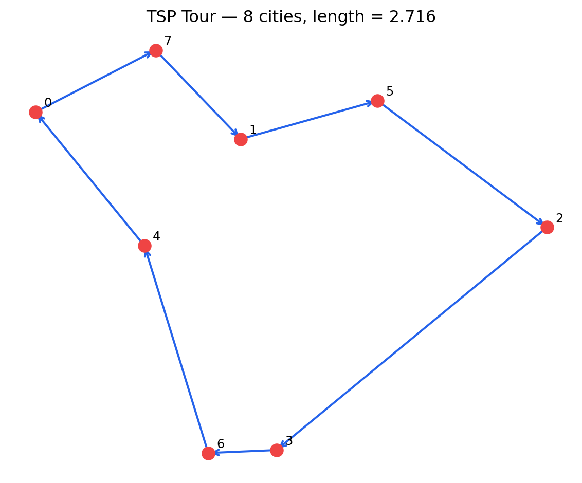
## The Travelling Salesman Problem {#sec-tsp}
The **Travelling Salesman Problem (TSP)** is the most famous combinatorial optimisation
problem: given $n$ cities and pairwise distances, find the shortest tour visiting every
city exactly once and returning to the start.
TSP is **NP-hard** — no polynomial-time exact algorithm is known for the general case.
Yet it is solvable in practice for hundreds or thousands of cities using IP with
specialised cutting planes (Subtour Elimination Constraints).
### Formulation
Let $x_{ij} \in \{0,1\}$: 1 if the tour goes directly from city $i$ to city $j$.
$$\text{Minimize} \quad \sum_{i \neq j} d_{ij} x_{ij}$$
$$\text{s.t.} \quad \sum_{j \neq i} x_{ij} = 1 \quad \forall i \quad \text{(leave each city once)}$$
$$\sum_{i \neq j} x_{ij} = 1 \quad \forall j \quad \text{(enter each city once)}$$
Plus **subtour elimination constraints** to prevent disconnected cycles.
```{python}
#| label: tsp-small
import pulp
import itertools
import numpy as np
import matplotlib.pyplot as plt

np.random.seed(7)
n = 8
coords = np.random.rand(n, 2)

# Distance matrix
dist = {(i, j): np.linalg.norm(coords[i] - coords[j])
        for i in range(n) for j in range(n) if i != j}

model = pulp.LpProblem("TSP", pulp.LpMinimize)

x = {(i, j): pulp.LpVariable(f"x_{i}_{j}", cat="Binary")
     for i in range(n) for j in range(n) if i != j}

# Objective
model += pulp.lpSum(dist[i, j] * x[i, j] for i, j in x), "Distance"

# Enter and leave each city exactly once
for i in range(n):
    model += pulp.lpSum(x[i, j] for j in range(n) if j != i) == 1, f"Leave_{i}"
    model += pulp.lpSum(x[j, i] for j in range(n) if j != i) == 1, f"Enter_{i}"

# Subtour elimination (Miller-Tucker-Zemlin formulation)
u = {i: pulp.LpVariable(f"u_{i}", lowBound=1, upBound=n - 1, cat="Continuous")
     for i in range(1, n)}

for i in range(1, n):
    for j in range(1, n):
        if i != j:
            model += u[i] - u[j] + (n - 1) * x[i, j] <= n - 2, f"MTZ_{i}_{j}"

model.solve(pulp.PULP_CBC_CMD(msg=0))

# Extract tour
tour = [0]
current = 0
for _ in range(n - 1):
    nxt = next(j for j in range(n) if j != current and pulp.value(x[current, j]) > 0.5)
    tour.append(nxt)
    current = nxt
tour.append(0)

total_dist = sum(dist[tour[k], tour[k+1]] for k in range(n))
print(f"Tour   : {' → '.join(str(c) for c in tour)}")
print(f"Length : {total_dist:.4f}")

# Plot
fig, ax = plt.subplots(figsize=(6, 5))
for k in range(len(tour) - 1):
    a, b = tour[k], tour[k + 1]
    ax.annotate("", xy=coords[b], xytext=coords[a],
                arrowprops=dict(arrowstyle="->", color="#2563eb", lw=1.5))
ax.scatter(coords[:, 0], coords[:, 1], s=80, color="#ef4444", zorder=3)
for i in range(n):
    ax.annotate(str(i), coords[i], textcoords="offset points",
                xytext=(6, 4), fontsize=9)
ax.set_title(f"TSP Tour — {n} cities, length = {total_dist:.3f}")
ax.axis("off")
plt.tight_layout()
plt.show()
```
For larger TSP instances, exact IP approaches (with lazy subtour elimination) or
meta-heuristics (simulated annealing, genetic algorithms) are preferred. The Google OR-Tools
library provides state-of-the-art TSP solvers.
---
## Common Modelling Patterns {#sec-patterns}
| Goal | Binary Formulation |
|---|---|
| Select exactly $k$ items | $\sum y_i = k$ |
| Select at most $k$ items | $\sum y_i \leq k$ |
| A requires B | $y_A \leq y_B$ |
| At most one of A, B | $y_A + y_B \leq 1$ |
| If $x > 0$ then $y = 1$ | $x \leq M \cdot y$ |
| Fixed charge (pay $f$ to use resource) | $f \cdot y + c \cdot x$ in objective; $x \leq M \cdot y$ |
Mastering these patterns — and combining them — is the core craft of IP modelling.
---
## Practical Guidance {#sec-ip-guidance}
**Start with the LP relaxation.** Solve without integrality and examine the fractional
variables. This reveals the structure of the problem and gives an optimality bound.
**Tighten the formulation.** Weak formulations (loose bounds on $M$, redundant
constraints) slow the solver by producing poor relaxation bounds. Better formulations
lead to tighter LP bounds and fewer Branch and Bound nodes.
**Limit solve time for large problems.** Real-world MIPs may not solve to provable
optimality in reasonable time. Set a time limit and accept the best solution found,
together with its **optimality gap** (how far the best integer solution is from the
LP bound).
```python
# Accept solution within 1% of optimal, or after 60 seconds
model.solve(pulp.PULP_CBC_CMD(msg=0, gapRel=0.01, timeLimit=60))
```
---
## Chapter Summary {#sec-ip-summary}
- Integer Programming adds integrality requirements to LP, capturing decisions that are
inherently discrete
- Binary variables are the primary modelling tool: they encode yes/no choices and
represent logical relationships (dependencies, exclusivity, fixed charges) as linear
constraints
- **Branch and Bound** solves IPs by systematically exploring a tree of LP relaxations,
pruning branches that cannot improve the current best solution
- Modern solvers combine Branch and Bound with cutting planes, presolving, and heuristics
to handle large-scale MIPs efficiently
- PuLP exposes integer and binary variables via `cat="Integer"` and `cat="Binary"` with
no change to the modelling interface
- Common patterns — selection, dependency, fixed charge — compose into powerful
formulations for facility location, scheduling, routing, and capital allocation