A History of Mathematical Optimization from Fermat to Karmarkar
Author
Troy Altus
Published
December 31, 2025
NoteLearning Objectives
Understand what optimization means as a mathematical discipline
Trace the isoperimetric problem from ancient Greece to modern engineering
See how Fermat’s method of stationary points planted the seed of calculus-based optimization
Recognize optimization as a unifying thread across disparate fields
Queen Dido’s Problem
According to Virgil, when the Phoenician princess Dido arrived on the coast of North Africa around 900 BCE, she struck a bargain with the local king. She could have as much land as she could enclose with a single oxhide. Dido cut the hide into thin strips, joined them end to end, and used the resulting length of leather to enclose a semicircle against the sea. She got more land than the king intended to give.
Whether or not Dido existed, the problem she solved is real. Given a fixed length of rope, what shape encloses the maximum area? The answer — a circle — was known empirically by the ancient Greeks, suspected to be true for centuries, and not proved rigorously until 1838, when the Swiss mathematician Jakob Steiner published five different proofs, all beautiful, all flawed. The first complete proof came from Karl Weierstrass in 1870, using a technique that would not be fully developed until the twentieth century.
The isoperimetric problem — equal perimeter, maximum area — is the oldest optimization problem in mathematics. It has a clean answer, a compelling physical interpretation, and a proof that eluded some of the greatest mathematicians of the nineteenth century. It also captures, in a single sentence, what optimization is about: given a constraint, find the best.
What Optimization Means
Optimization, as a mathematical discipline, asks a specific question: given a function \(f(\mathbf{x})\) and a set of constraints, find the value of \(\mathbf{x}\) that makes \(f\) as small (or as large) as possible.
The function \(f\) is called the objective. The constraints define the feasible set — the region of valid solutions. The solution, if it exists, is the optimum. These three elements — objective, feasible set, optimum — appear in every optimization problem from Dido’s oxhide to a solid rocket motor grain design.
The simplicity of this formulation is deceptive. The objective might be smooth and convex, in which case the optimum is unique and easy to find. Or it might be riddled with local minima, discontinuous, noisy, or defined only implicitly through a simulation code. The feasible set might be a simple box, a complicated surface in high-dimensional space, or a discrete set of integers. The optimum might be well-defined and easy to characterize, or it might not exist at all.
The history of optimization is largely a history of mathematicians learning to handle these complications — extending the simple idea of finding a minimum to cover the full range of problems that the physical and economic world actually presents.
Fermat and the Stationary Point
The first systematic technique for finding optima arrived in the seventeenth century, before calculus existed as a unified subject. Pierre de Fermat, the French lawyer and amateur mathematician who is better known for his work in number theory, noticed something about the maximum of a function.
Consider a parabola opening downward, reaching its peak at some point \(x^*\). At the peak, the tangent is horizontal — the function neither rises nor falls. Fermat formalized this observation: at an interior maximum or minimum of a smooth function, the derivative is zero. This is Fermat’s theorem on stationary points, and it is the foundation of every gradient-based optimization method that has ever been invented.
Fermat stated his result in 1638, in the language of algebraic geometry rather than calculus, but the idea is unmistakably modern. He wrote that at the point of maximum or minimum, the value of the function is “adequal” to its value at a nearby point — meaning the difference is negligible. Substitute \(x + \epsilon\) for \(x\), compute the expression, set the terms involving \(\epsilon\) to zero, and solve. This is essentially the method of setting the derivative equal to zero, discovered before the derivative had a formal definition.
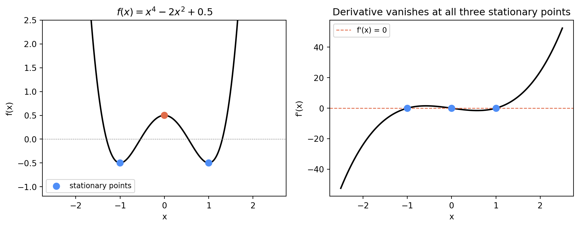
Isaac Newton and Gottfried Leibniz formalized Fermat’s intuition into calculus in the 1660s and 1670s. The machinery of derivatives made Fermat’s method precise: a necessary condition for an interior minimum or maximum of a differentiable function is that the derivative vanishes. The condition is necessary but not sufficient — it identifies candidates (stationary points) but does not distinguish minima from maxima or saddle points. Distinguishing these requires the second derivative.
Figure 1: Fermat’s stationary point condition: at every local minimum or maximum, the derivative is zero. The derivative is zero at saddle points too — the condition is necessary, not sufficient.
The Brachistochrone Problem and What It Started
In 1696, Johann Bernoulli posed the brachistochrone problem in the pages of the journal Acta Eruditorum. A bead slides without friction along a wire connecting two points. What shape should the wire take to minimize the time of descent?
The problem is phrased as a challenge: “I, Johann Bernoulli, address the most brilliant mathematicians in the world. Nothing is more attractive to intelligent people than an honest, challenging problem whose possible solution will bestow fame and remain as a lasting monument.”
Five solutions arrived within a year. Newton solved it overnight, anonymously, but Bernoulli recognized his style: “I recognize the lion by his paw.” Leibniz, Jakob Bernoulli (Johann’s older brother), and the Marquis de l’Hôpital also submitted solutions. The answer was the cycloid — the curve traced by a point on the rim of a rolling circle.
The brachistochrone problem was not just a clever puzzle. It was the opening move in the development of the calculus of variations, the branch of mathematics that asks: among all possible functions, which one minimizes a given integral? This is optimization over an infinite-dimensional space — not “find the best value of \(x\)” but “find the best function\(y(x)\).” It is a profound generalization, and it set the agenda for mathematical physics for two centuries.
Optimization as a Unifying Principle
What makes the history of optimization unusual is how many different fields converged on the same mathematical ideas from completely different directions.
Natural philosophers asked why nature seemed to be economical. Fermat’s principle of least time says light takes the path that minimizes travel time. Hamilton’s principle says a mechanical system follows the path that minimizes the integral of kinetic minus potential energy — the action. Minimum energy, minimum time, minimum cost: the physical world seemed to be optimizing something, and finding what it was minimizing revealed the governing equations.
Economists asked how to allocate limited resources. The question of maximizing utility subject to a budget constraint, or minimizing cost subject to production requirements, turned out to require the same mathematical machinery as finding the minimum of a function subject to inequality constraints.
Engineers asked how to design structures, machines, and systems that were as good as possible within given constraints — minimize weight, maximize strength, minimize propellant mass while meeting performance requirements. The same KKT conditions that describe the optimal allocation of resources in an economy describe the optimal shape of a rocket motor grain.
Military planners, after World War II, asked how to route supplies, schedule operations, and allocate equipment as efficiently as possible. The result was linear programming — the most widely used optimization technique in the world, handling millions of variables and constraints in every major airline, shipping company, and manufacturing firm on earth.
The common thread is the gradient. Whether you are finding the stationary point of a function, minimizing an integral over curves, satisfying complementary slackness conditions, or following the central path of an interior point method, you are always asking the same question in different notation: in which direction does the objective improve, and how far should we go?
The Chapters Ahead
The story begins with the brachistochrone and the calculus of variations — the first systematic framework for optimization over function spaces. From there it moves to Lagrange’s multiplier, the idea that constrained optimization can be converted to unconstrained optimization by augmenting the objective. Then to Cauchy’s steepest descent algorithm of 1847, the first numerical optimization method, rediscovered repeatedly for a century before it became the workhorse of machine learning.
The middle section covers the twentieth-century explosion: Dantzig’s simplex method for linear programming, born in the war rooms and operations research centers of 1940s America; Kantorovich’s independent discovery of the same ideas in Soviet Russia; and the Kuhn-Tucker conditions for nonlinear programming, which unified constrained optimization theory under a single framework.
The final chapters cover the interior point revolution — Karmarkar’s 1984 result that changed the complexity of linear programming and eventually produced the solvers running in every modern engineering tool — and the modern landscape of nonlinear optimization, surrogate methods, and the strange return of gradient descent as the dominant algorithm of an era of machine learning.
The gradient runs through all of it.
Summary
Optimization asks a single question — find the best — and the diversity of contexts in which that question arises has driven the development of mathematics for three centuries. The isoperimetric problem posed by Dido’s legend is structurally identical to the grain geometry optimization problem on a modern engineer’s workstation. Fermat’s observation about stationary points is the ancestor of every gradient-based algorithm. The brachistochrone problem opened the door to the calculus of variations and, through it, to the entire modern theory of optimal control.
The history ahead is a story of ideas generalizing — from functions to functionals, from unconstrained to constrained, from equality constraints to inequality constraints, from smooth to nonsmooth, from small problems solvable by hand to large problems solvable only by computers. Each generalization required new mathematics, and each piece of new mathematics opened new applications.
Further Reading
Goldstine (1980) is the definitive history of the calculus of variations, tracing the mathematical development from Bernoulli to Weierstrass with full technical detail. Nocedal and Wright (2006) provides modern context: Chapter 1 situates the algorithms of this book within the broader landscape. For the isoperimetric problem specifically, Osserman’s A Survey of Minimal Surfaces (Dover, 1986) gives a rigorous but readable treatment.
Goldstine, Herman H. 1980. A History of the Calculus of Variations from the 17th Through the 19th Century. Springer.
Nocedal, Jorge, and Stephen J. Wright. 2006. Numerical Optimization. 2nd ed. Springer.
Source Code
---title: "The Shape of the Possible"number-sections: false---::: {.callout-note}## Learning Objectives- Understand what optimization means as a mathematical discipline- Trace the isoperimetric problem from ancient Greece to modern engineering- See how Fermat's method of stationary points planted the seed of calculus-based optimization- Recognize optimization as a unifying thread across disparate fields:::## Queen Dido's ProblemAccording to Virgil, when the Phoenician princess Dido arrived on the coast of North Africa around 900 BCE, she struck a bargain with the local king. She could have as much land as she could enclose with a single oxhide. Dido cut the hide into thin strips, joined them end to end, and used the resulting length of leather to enclose a semicircle against the sea. She got more land than the king intended to give.Whether or not Dido existed, the problem she solved is real. Given a fixed length of rope, what shape encloses the maximum area? The answer — a circle — was known empirically by the ancient Greeks, suspected to be true for centuries, and not proved rigorously until 1838, when the Swiss mathematician Jakob Steiner published five different proofs, all beautiful, all flawed. The first complete proof came from Karl Weierstrass in 1870, using a technique that would not be fully developed until the twentieth century.The isoperimetric problem — *equal perimeter, maximum area* — is the oldest optimization problem in mathematics. It has a clean answer, a compelling physical interpretation, and a proof that eluded some of the greatest mathematicians of the nineteenth century. It also captures, in a single sentence, what optimization is about: given a constraint, find the best.## What Optimization MeansOptimization, as a mathematical discipline, asks a specific question: given a function $f(\mathbf{x})$ and a set of constraints, find the value of $\mathbf{x}$ that makes $f$ as small (or as large) as possible.The function $f$ is called the *objective*. The constraints define the *feasible set* — the region of valid solutions. The solution, if it exists, is the *optimum*. These three elements — objective, feasible set, optimum — appear in every optimization problem from Dido's oxhide to a solid rocket motor grain design.The simplicity of this formulation is deceptive. The objective might be smooth and convex, in which case the optimum is unique and easy to find. Or it might be riddled with local minima, discontinuous, noisy, or defined only implicitly through a simulation code. The feasible set might be a simple box, a complicated surface in high-dimensional space, or a discrete set of integers. The optimum might be well-defined and easy to characterize, or it might not exist at all.The history of optimization is largely a history of mathematicians learning to handle these complications — extending the simple idea of finding a minimum to cover the full range of problems that the physical and economic world actually presents.## Fermat and the Stationary PointThe first systematic technique for finding optima arrived in the seventeenth century, before calculus existed as a unified subject. Pierre de Fermat, the French lawyer and amateur mathematician who is better known for his work in number theory, noticed something about the maximum of a function.Consider a parabola opening downward, reaching its peak at some point $x^*$. At the peak, the tangent is horizontal — the function neither rises nor falls. Fermat formalized this observation: at an interior maximum or minimum of a smooth function, the derivative is zero. This is Fermat's theorem on stationary points, and it is the foundation of every gradient-based optimization method that has ever been invented.Fermat stated his result in 1638, in the language of algebraic geometry rather than calculus, but the idea is unmistakably modern. He wrote that at the point of maximum or minimum, the value of the function is "adequal" to its value at a nearby point — meaning the difference is negligible. Substitute $x + \epsilon$ for $x$, compute the expression, set the terms involving $\epsilon$ to zero, and solve. This is essentially the method of setting the derivative equal to zero, discovered before the derivative had a formal definition.Isaac Newton and Gottfried Leibniz formalized Fermat's intuition into calculus in the 1660s and 1670s. The machinery of derivatives made Fermat's method precise: a necessary condition for an interior minimum or maximum of a differentiable function is that the derivative vanishes. The condition is necessary but not sufficient — it identifies candidates (stationary points) but does not distinguish minima from maxima or saddle points. Distinguishing these requires the second derivative.```{python}#| label: fig-fermat-stationary#| fig-cap: "Fermat's stationary point condition: at every local minimum or maximum, the derivative is zero. The derivative is zero at saddle points too — the condition is necessary, not sufficient."import numpy as npimport matplotlib.pyplot as pltx = np.linspace(-2.5, 2.5, 400)f = x**4-2*x**2+0.5fig, axes = plt.subplots(1, 2, figsize=(10, 4))# Left: function with stationary points markedax = axes[0]ax.plot(x, f, 'k-', linewidth=1.8)stationary_x = np.array([-1, 0, 1])stationary_f = stationary_x**4-2*stationary_x**2+0.5ax.scatter(stationary_x, stationary_f, s=60, zorder=5, color=['#4f8ef7', '#e06c4a', '#4f8ef7'], label='stationary points')ax.axhline(0, color='gray', linewidth=0.5, linestyle='--')ax.set_xlabel('x')ax.set_ylabel('f(x)')ax.set_title("$f(x) = x^4 - 2x^2 + 0.5$")ax.legend(fontsize=9)ax.set_ylim(-1.2, 2.5)# Right: derivativedf =4*x**3-4*xax = axes[1]ax.plot(x, df, 'k-', linewidth=1.8)ax.axhline(0, color='#e06c4a', linewidth=1, linestyle='--', label="f'(x) = 0")ax.scatter(stationary_x, [0,0,0], s=60, zorder=5, color='#4f8ef7')ax.set_xlabel('x')ax.set_ylabel("f'(x)")ax.set_title("Derivative vanishes at all three stationary points")ax.legend(fontsize=9)plt.tight_layout()plt.savefig('figures/fermat_stationary.png', dpi=150, bbox_inches='tight')plt.show()```## The Brachistochrone Problem and What It StartedIn 1696, Johann Bernoulli posed the brachistochrone problem in the pages of the journal *Acta Eruditorum*. A bead slides without friction along a wire connecting two points. What shape should the wire take to minimize the time of descent?The problem is phrased as a challenge: "I, Johann Bernoulli, address the most brilliant mathematicians in the world. Nothing is more attractive to intelligent people than an honest, challenging problem whose possible solution will bestow fame and remain as a lasting monument."Five solutions arrived within a year. Newton solved it overnight, anonymously, but Bernoulli recognized his style: "I recognize the lion by his paw." Leibniz, Jakob Bernoulli (Johann's older brother), and the Marquis de l'Hôpital also submitted solutions. The answer was the cycloid — the curve traced by a point on the rim of a rolling circle.The brachistochrone problem was not just a clever puzzle. It was the opening move in the development of the *calculus of variations*, the branch of mathematics that asks: among all possible functions, which one minimizes a given integral? This is optimization over an infinite-dimensional space — not "find the best value of $x$" but "find the best *function* $y(x)$." It is a profound generalization, and it set the agenda for mathematical physics for two centuries.## Optimization as a Unifying PrincipleWhat makes the history of optimization unusual is how many different fields converged on the same mathematical ideas from completely different directions.Natural philosophers asked why nature seemed to be economical. Fermat's principle of least time says light takes the path that minimizes travel time. Hamilton's principle says a mechanical system follows the path that minimizes the integral of kinetic minus potential energy — the *action*. Minimum energy, minimum time, minimum cost: the physical world seemed to be optimizing something, and finding what it was minimizing revealed the governing equations.Economists asked how to allocate limited resources. The question of maximizing utility subject to a budget constraint, or minimizing cost subject to production requirements, turned out to require the same mathematical machinery as finding the minimum of a function subject to inequality constraints.Engineers asked how to design structures, machines, and systems that were as good as possible within given constraints — minimize weight, maximize strength, minimize propellant mass while meeting performance requirements. The same KKT conditions that describe the optimal allocation of resources in an economy describe the optimal shape of a rocket motor grain.Military planners, after World War II, asked how to route supplies, schedule operations, and allocate equipment as efficiently as possible. The result was linear programming — the most widely used optimization technique in the world, handling millions of variables and constraints in every major airline, shipping company, and manufacturing firm on earth.The common thread is the gradient. Whether you are finding the stationary point of a function, minimizing an integral over curves, satisfying complementary slackness conditions, or following the central path of an interior point method, you are always asking the same question in different notation: in which direction does the objective improve, and how far should we go?## The Chapters AheadThe story begins with the brachistochrone and the calculus of variations — the first systematic framework for optimization over function spaces. From there it moves to Lagrange's multiplier, the idea that constrained optimization can be converted to unconstrained optimization by augmenting the objective. Then to Cauchy's steepest descent algorithm of 1847, the first numerical optimization method, rediscovered repeatedly for a century before it became the workhorse of machine learning.The middle section covers the twentieth-century explosion: Dantzig's simplex method for linear programming, born in the war rooms and operations research centers of 1940s America; Kantorovich's independent discovery of the same ideas in Soviet Russia; and the Kuhn-Tucker conditions for nonlinear programming, which unified constrained optimization theory under a single framework.The final chapters cover the interior point revolution — Karmarkar's 1984 result that changed the complexity of linear programming and eventually produced the solvers running in every modern engineering tool — and the modern landscape of nonlinear optimization, surrogate methods, and the strange return of gradient descent as the dominant algorithm of an era of machine learning.The gradient runs through all of it.---## SummaryOptimization asks a single question — find the best — and the diversity of contexts in which that question arises has driven the development of mathematics for three centuries. The isoperimetric problem posed by Dido's legend is structurally identical to the grain geometry optimization problem on a modern engineer's workstation. Fermat's observation about stationary points is the ancestor of every gradient-based algorithm. The brachistochrone problem opened the door to the calculus of variations and, through it, to the entire modern theory of optimal control.The history ahead is a story of ideas generalizing — from functions to functionals, from unconstrained to constrained, from equality constraints to inequality constraints, from smooth to nonsmooth, from small problems solvable by hand to large problems solvable only by computers. Each generalization required new mathematics, and each piece of new mathematics opened new applications.## Further Reading@goldstine1980history is the definitive history of the calculus of variations, tracing the mathematical development from Bernoulli to Weierstrass with full technical detail. @nocedal2006numerical provides modern context: Chapter 1 situates the algorithms of this book within the broader landscape. For the isoperimetric problem specifically, Osserman's *A Survey of Minimal Surfaces* (Dover, 1986) gives a rigorous but readable treatment.