---
title: "The Machine Learns to Optimize"
---
::: {.callout-note}
## Learning Objectives
- Understand backpropagation as automatic differentiation through a computational graph
- See how stochastic gradient descent (Cauchy's algorithm) became the engine of deep learning
- Understand the Adam optimizer and why it dominates neural network training
- Reflect on how optimization connects classical engineering to modern AI
:::
## Cauchy's Algorithm, One More Time
In 2012, Geoffrey Hinton, Ilya Sutskever, and Alex Krizhevsky trained a convolutional neural network called AlexNet using a GPU cluster at the University of Toronto. AlexNet won the ImageNet Large Scale Visual Recognition Challenge by a margin that stunned the computer vision community — it achieved 15.3% top-5 error, compared to 26.2% for the next-best entry. The field changed overnight.
AlexNet was trained using stochastic gradient descent: start at a random point in a space with 60 million dimensions, and iterate $\mathbf{x}_{k+1} = \mathbf{x}_k - \alpha_k \hat{\nabla} f(\mathbf{x}_k)$, where $\hat{\nabla} f$ is the gradient estimated from a random mini-batch of training data. This is Augustin-Louis Cauchy's 1847 algorithm, applied to a function with sixty million variables, trained on one million images.
Nothing in Cauchy's paper would have predicted this. The zigzag convergence problem that makes steepest descent slow on ill-conditioned quadratics is also present in neural network training, but it matters less because neural networks are so overparameterized — the loss landscape is so flat in so many directions — that any reasonable descent direction makes progress. The noise introduced by mini-batch sampling turns out to help, not hurt, by preventing the optimizer from settling into sharp, narrow minima that generalize poorly.
## Backpropagation: The Gradient Machine
Training a neural network requires computing the gradient of the loss function with respect to all parameters. For a network with 60 million parameters, computing this gradient by finite differences would require 60 million forward passes — computationally catastrophic.
Backpropagation, popularized by Rumelhart, Hinton, and Williams in their 1986 *Nature* paper (and independently discovered by several others earlier), is the efficient solution. It computes the exact gradient of any differentiable function defined by a computational graph using the chain rule, in time proportional to the cost of a single forward evaluation.
The key insight: the chain rule can be applied in reverse order, propagating gradient information from the output backward through the network. Each layer computes a local Jacobian; multiplying these Jacobians together gives the full gradient. The total cost is two forward passes (one forward, one backward), regardless of the number of parameters.
Backpropagation is, mathematically, the adjoint method applied to feedforward neural networks. The adjoint method — covered in the optimization lesson series — is the same algorithm applied to partial differential equations and used in aerodynamic shape optimization and solid rocket motor sensitivity analysis. The deep learning community and the computational fluid dynamics community independently developed the same idea for different applications.
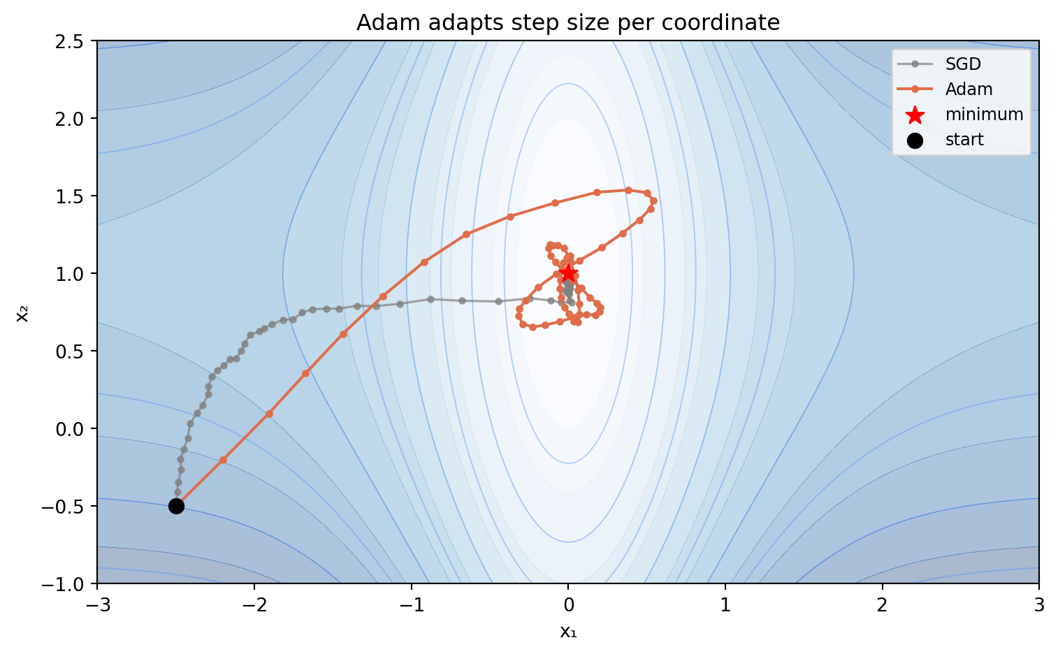
## Adam: The Modern SGD
Stochastic gradient descent with a fixed learning rate performs poorly in practice — the learning rate that works early in training (when far from the optimum) is too large late in training (when near the optimum), and vice versa. Adapting the learning rate to the local geometry of the loss function was the key practical advance of the 2010s.
The Adam optimizer (Kingma and Ba, 2015) maintains running estimates of the first and second moments of the gradient:
$$m_k = \beta_1 m_{k-1} + (1-\beta_1)\hat{\nabla} f_k$$
$$v_k = \beta_2 v_{k-1} + (1-\beta_2)\hat{\nabla} f_k^2$$
After bias correction ($\hat{m}_k = m_k/(1-\beta_1^k)$, $\hat{v}_k = v_k/(1-\beta_2^k)$), the update is:
$$\mathbf{x}_{k+1} = \mathbf{x}_k - \frac{\alpha}{\sqrt{\hat{v}_k} + \epsilon}\hat{m}_k$$
The denominator $\sqrt{\hat{v}_k}$ acts as a per-parameter learning rate scaler: parameters with large recent gradients (likely in a steep direction) get smaller steps; parameters with small recent gradients get larger steps. This is an adaptive preconditioner — a poor man's Newton step that avoids computing the full Hessian.
```{python}
#| label: fig-adam-vs-sgd
#| fig-cap: "Adam vs. SGD with fixed learning rate on a simple non-convex function. Adam adapts its effective step size per coordinate, navigating the flat plateau more efficiently than fixed-rate SGD. The advantage is most pronounced in high dimensions and near flat regions."
import numpy as np
import matplotlib.pyplot as plt

np.random.seed(42)

def f(x):
    return np.tanh(x[0])**2 + 0.1*(x[1]-1)**2

def grad_f(x, noise_scale=0.05):
    g0 = 2*np.tanh(x[0])*(1-np.tanh(x[0])**2) + np.random.randn()*noise_scale
    g1 = 0.2*(x[1]-1) + np.random.randn()*noise_scale
    return np.array([g0, g1])

def sgd(x0, lr=0.3, n=60):
    x = x0.copy()
    path = [x.copy()]
    for _ in range(n):
        g = grad_f(x)
        x = x - lr*g
        path.append(x.copy())
    return np.array(path)

def adam(x0, lr=0.3, n=60, b1=0.9, b2=0.999, eps=1e-8):
    x = x0.copy()
    m, v = np.zeros(2), np.zeros(2)
    path = [x.copy()]
    for t in range(1, n+1):
        g = grad_f(x)
        m = b1*m + (1-b1)*g
        v = b2*v + (1-b2)*g**2
        mh = m/(1-b1**t)
        vh = v/(1-b2**t)
        x = x - lr*mh/(np.sqrt(vh)+eps)
        path.append(x.copy())
    return np.array(path)

x0 = np.array([-2.5, -0.5])
p_sgd = sgd(x0)
p_adam = adam(x0)

x = np.linspace(-3, 3, 200)
y = np.linspace(-1, 2.5, 200)
X, Y = np.meshgrid(x, y)
Z = np.tanh(X)**2 + 0.1*(Y-1)**2

fig, ax = plt.subplots(figsize=(8, 5))
ax.contourf(X, Y, Z, levels=15, cmap='Blues', alpha=0.35)
ax.contour(X, Y, Z, levels=10, colors='#4f8ef7', alpha=0.4, linewidths=0.7)
ax.plot(p_sgd[:,0], p_sgd[:,1], 'o-', color='gray', markersize=3, linewidth=1.2, label='SGD', alpha=0.7)
ax.plot(p_adam[:,0], p_adam[:,1], 'o-', color='#e06c4a', markersize=3, linewidth=1.5, label='Adam', zorder=4)
ax.scatter([0], [1], s=100, color='red', zorder=6, marker='*', label='minimum')
ax.scatter(*x0, s=60, color='k', zorder=5, label='start')
ax.set_xlabel('x₁')
ax.set_ylabel('x₂')
ax.set_title('Adam adapts step size per coordinate')
ax.legend(fontsize=9)
plt.tight_layout()
plt.savefig('figures/adam_vs_sgd.png', dpi=150, bbox_inches='tight')
plt.show()
```
## Bayesian Optimization: When Evaluations Are Expensive
For problems where the objective function is expensive to evaluate — a neural architecture search requiring days of GPU training, an aerodynamic shape requiring hours of CFD simulation, a propellant formulation requiring synthesis and testing — gradient descent is impractical. The function is a black box; derivatives may be unavailable; and the budget of evaluations is measured in dozens, not millions.
Bayesian optimization treats the objective as a sample from a Gaussian process prior, updates the posterior after each evaluation, and uses an *acquisition function* to decide where to evaluate next. The acquisition function balances exploration (evaluating where uncertainty is high) and exploitation (evaluating where the posterior mean is low). The most common acquisition function is expected improvement (EI): the expected reduction in the best value seen so far.
Bayesian optimization is provably sample-efficient for smooth functions, achieving sublinear cumulative regret under mild assumptions on the Gaussian process kernel. In practice, it typically finds good solutions in 50–200 evaluations on problems where gradient methods would need thousands. It is now the standard method for hyperparameter tuning in machine learning.
## The Gradient Runs Through It
Looking back at the three centuries covered by this book, one thread runs through everything: the gradient.
Fermat's stationary points. Euler's first variation. Lagrange's multiplier. Cauchy's steepest descent. Dantzig's reduced costs. Kantorovich's resolving multipliers. The KKT gradient condition. Karmarkar's projective step. IPOPT's Newton iteration. Adam's adaptive gradient. Backpropagation's chain rule.
Every one of these is, at its core, a statement about the gradient of some function — where it vanishes, how to follow it, how to project it, how to modify it, how to combine it with constraint information. The field changes its notation every generation, but the mathematics is recognizably the same mathematics that Cauchy wrote down in two pages in 1847.
The problems change. Lagrange was minimizing the potential energy of a mechanical system. Dantzig was allocating Air Force resources. Hinton was classifying images. The researchers currently using neural networks to fold proteins, predict weather, and design drugs are solving optimization problems that Lagrange could not have imagined. The gradient — his gradient, Cauchy's gradient — is what makes it possible.
---
## Summary
Stochastic gradient descent — Cauchy's 1847 algorithm applied to functions with millions of variables — became the engine of the deep learning revolution. Backpropagation computes exact gradients efficiently through the chain rule applied in reverse, enabling training of networks with billions of parameters. Adam's adaptive step sizing addresses the ill-conditioning problem that afflicts basic gradient descent. Bayesian optimization handles the black-box setting where evaluations are expensive. The thread connecting all of these methods to the history of optimization is the gradient — the fundamental concept introduced by Cauchy and refined by every chapter in between.
## Further Reading
Rumelhart, Hinton, and Williams' "Learning representations by back-propagating errors" (*Nature*, 323:533–536, 1986) is the backpropagation paper. Kingma and Ba's "Adam: A method for stochastic optimization" (ICLR 2015) introduces Adam. Frazier's "A tutorial on Bayesian optimization" (arXiv:1807.02811, 2018) is the best accessible introduction to Bayesian optimization. For the deep learning context generally, Goodfellow, Bengio, and Courville's *Deep Learning* (MIT Press, 2016) is the standard reference; Chapter 8 covers gradient-based optimization in depth.