---
title: "Going Downhill"
---
::: {.callout-note}
## Learning Objectives
- Understand Cauchy's steepest descent algorithm and its 1847 origins
- Analyze convergence behavior and the zigzag phenomenon
- Understand why steepest descent was rediscovered repeatedly for a century
- Connect the historical algorithm to modern gradient descent in machine learning
:::
## Cauchy's Throwaway Result
In 1847, Augustin-Louis Cauchy published a short paper in the *Comptes Rendus de l'Académie des Sciences* with the title "Méthode générale pour la résolution des systèmes d'équations simultanées" — General method for the resolution of systems of simultaneous equations. The paper presented what we now call the steepest descent algorithm as a side result, mentioned almost in passing. Cauchy did not follow up on it. He did not analyze its convergence. He did not apply it to any interesting problem.
He had, however, invented the method that would become the most important algorithm in the history of machine learning, used today to train every large neural network on earth.
The algorithm is simple: to minimize a function $f(\mathbf{x})$, start at some point $\mathbf{x}_0$ and repeatedly move in the direction of the negative gradient:
$$\mathbf{x}_{k+1} = \mathbf{x}_k - \alpha_k \nabla f(\mathbf{x}_k)$$
The gradient $\nabla f$ points uphill; its negative points downhill. The step size $\alpha_k$ (the learning rate, in modern parlance) controls how far to go. The idea is obvious in retrospect — go downhill — and its obvious simplicity obscured the nontrivial question of how fast it converges and when it fails.
## The Zigzag Problem
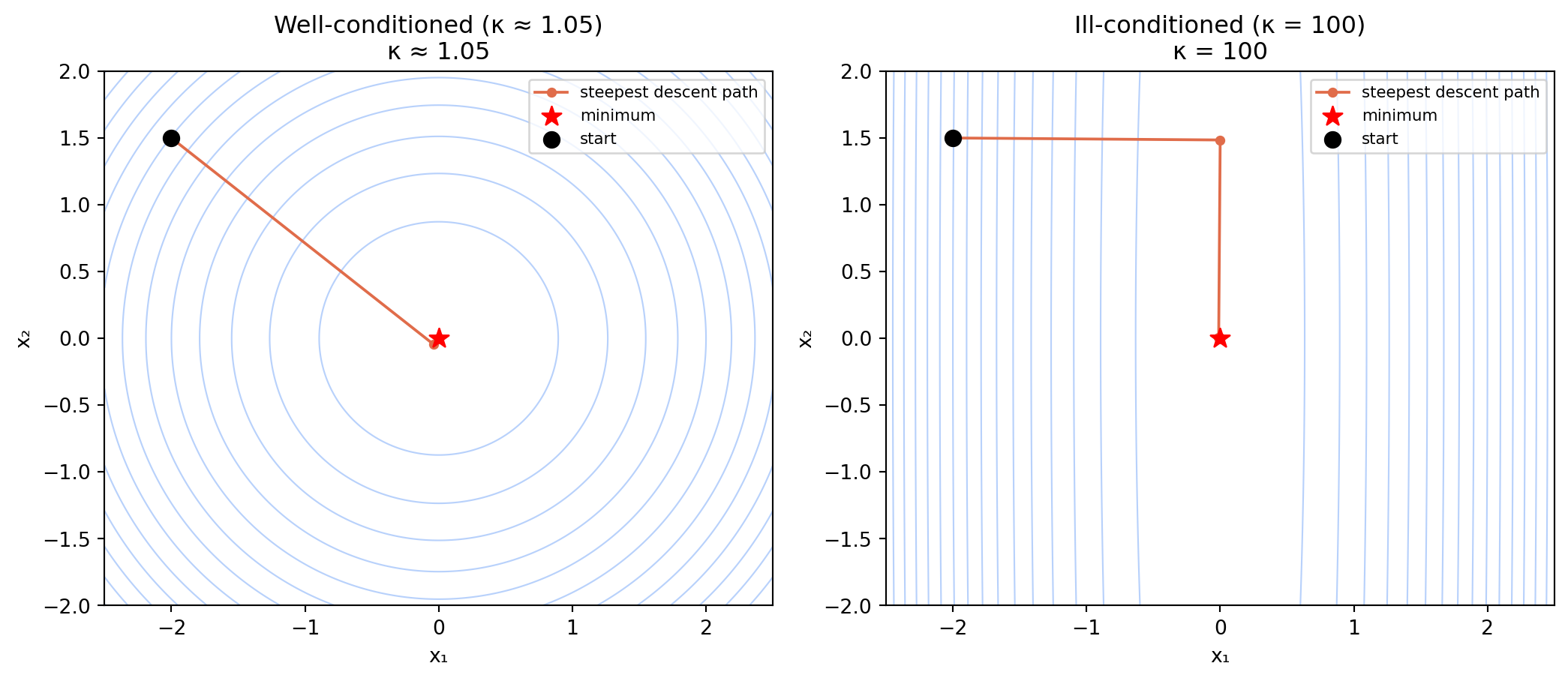
For a smooth, strongly convex function, steepest descent converges to the minimum. But the convergence can be painfully slow, and the reason is geometric.
Consider minimizing a quadratic $f(\mathbf{x}) = \frac{1}{2}\mathbf{x}^T A \mathbf{x} - \mathbf{b}^T \mathbf{x}$ where $A$ is symmetric positive definite. The level curves are ellipses. Steepest descent with exact line search takes steps that are exactly orthogonal at each iteration — the new gradient is perpendicular to the previous step. On a round ellipse (eigenvalues of $A$ close together), this works well. On a very elongated ellipse (eigenvalues far apart), the algorithm zigzags back and forth across the valley, making tiny net progress with each step.
The convergence rate depends on the *condition number* $\kappa = \lambda_{max}/\lambda_{min}$ — the ratio of largest to smallest eigenvalue of $A$. The error after $k$ iterations satisfies:
$$\|\mathbf{x}_k - \mathbf{x}^*\| \leq \left(\frac{\kappa - 1}{\kappa + 1}\right)^k \|\mathbf{x}_0 - \mathbf{x}^*\|$$
For $\kappa = 10$, the factor is $(9/11)^k \approx 0.82^k$ — slow. For $\kappa = 1000$, it is $(999/1001)^k \approx 0.998^k$ — catastrophically slow. This is the curse of ill-conditioning, and it is why steepest descent alone is almost never used for serious numerical optimization.
```{python}
#| label: fig-steepest-descent-zigzag
#| fig-cap: "Steepest descent on a well-conditioned (left) and ill-conditioned (right) quadratic. On the elongated ellipse, the algorithm zigzags, making tiny net progress toward the minimum (red star). The condition number κ governs the severity of the zigzag."
import numpy as np
import matplotlib.pyplot as plt

def steepest_descent(A, b, x0, n_steps=20, alpha=None):
    x = x0.copy().astype(float)
    path = [x.copy()]
    for _ in range(n_steps):
        g = A @ x - b
        if alpha is None:
            # Exact line search for quadratic
            a = (g @ g) / (g @ A @ g)
        else:
            a = alpha
        x = x - a * g
        path.append(x.copy())
    return np.array(path)

fig, axes = plt.subplots(1, 2, figsize=(11, 5))

for ax, (A, title, kappa_str) in zip(axes, [
    (np.array([[2., 0.], [0., 2.1]]), 'Well-conditioned (κ ≈ 1.05)', 'κ ≈ 1.05'),
    (np.array([[20., 0.], [0., 0.2]]), 'Ill-conditioned (κ = 100)', 'κ = 100')
]):
    b = np.array([0., 0.])
    x_opt = np.linalg.solve(A, b)
    x0 = np.array([-2., 1.5])

    path = steepest_descent(A, b, x0, n_steps=15)

    x = np.linspace(-2.5, 2.5, 300)
    y = np.linspace(-2., 2., 300)
    X, Y = np.meshgrid(x, y)
    Z = 0.5*(A[0,0]*X**2 + A[1,1]*Y**2)

    ax.contour(X, Y, Z, levels=15, colors='#4f8ef7', alpha=0.4, linewidths=0.8)
    ax.plot(path[:,0], path[:,1], 'o-', color='#e06c4a', markersize=4,
            linewidth=1.4, label='steepest descent path', zorder=4)
    ax.scatter(*x_opt, s=100, color='red', zorder=6, marker='*', label='minimum')
    ax.scatter(*x0, s=60, color='k', zorder=5, label='start')
    ax.set_title(f'{title}\n{kappa_str}')
    ax.set_xlim(-2.5, 2.5)
    ax.set_ylim(-2., 2.)
    ax.set_aspect('equal')
    ax.legend(fontsize=8)
    ax.set_xlabel('x₁')
    ax.set_ylabel('x₂')

plt.tight_layout()
plt.savefig('figures/steepest_descent_zigzag.png', dpi=150, bbox_inches='tight')
plt.show()
```
## A Century of Rediscovery
Cauchy's 1847 paper was largely forgotten. The method was rediscovered — independently and repeatedly — by mathematicians who did not know the prior work. The most important rediscovery was by Haskell Curry in 1944, working in the context of electronic computing. Curry wrote a technical report for the Ballistic Research Laboratory analyzing the convergence of gradient methods for solving systems of equations, unaware of Cauchy's paper.
The pattern of independent rediscovery is itself historically interesting. The steepest descent idea is simple enough to be reinvented from scratch by anyone who has thought carefully about the geometry of optimization, but it was not published in places where applied mathematicians would encounter it. The *Comptes Rendus* was not widely read outside France; Cauchy's paper was buried in his vast output; and the idea of numerical iterative methods was not yet a recognized field with its own literature.
The situation changed in the 1950s. The development of digital computers created a pressing demand for practical algorithms for solving large systems of equations and optimization problems. Gradient methods were rediscovered, analyzed, and published in journals that numerical analysts read. By 1960, the literature on gradient methods was growing rapidly, and the question of convergence rates — how fast the method approaches the minimum — was being attacked with serious mathematical tools.
## Conjugate Gradient: The Fix That Worked
The zigzag problem was solved in 1952 by Magnus Hestenes and Eduard Stiefel, working independently at the National Bureau of Standards and ETH Zürich. The conjugate gradient method chooses search directions that are mutually *conjugate* with respect to the Hessian matrix, meaning $\mathbf{d}_i^T A \mathbf{d}_j = 0$ for $i \neq j$. This property ensures that minimizing along each direction does not undo progress made along previous directions.
The result: for a quadratic function in $\mathbb{R}^n$, conjugate gradient finds the exact solution in at most $n$ steps. The zigzag is eliminated. For non-quadratic functions, conjugate gradient is used as an iterative method with restarts, and it remains one of the most efficient large-scale optimization algorithms known.
## The Machine Learning Connection
In 2012, Geoffrey Hinton and colleagues published the AlexNet neural network, which won the ImageNet image classification competition by a margin that stunned the computer vision community. AlexNet was trained using stochastic gradient descent — a variant of Cauchy's 1847 algorithm where the gradient is estimated from a random mini-batch of training data rather than the full dataset.
The irony is that the algorithm used to train the most consequential AI systems of the early twenty-first century was invented 165 years earlier as a footnote in a paper about solving linear systems. Cauchy did not think it was interesting. He was wrong.
The reason stochastic gradient descent works for neural network training is that neural networks are so overparameterized — they have far more parameters than data points — that noise in the gradient estimate is not a bug but a feature. The noise prevents the optimizer from settling into sharp, poorly-generalizing minima and encourages it toward flat, broad minima that generalize better. This is an empirical observation that is not yet fully understood theoretically, and it would have baffled Cauchy entirely.
---
## Summary
Steepest descent — moving in the direction of the negative gradient — is the oldest numerical optimization algorithm, invented by Cauchy in 1847 and rediscovered repeatedly for a century. It converges for smooth strongly convex functions but suffers from the zigzag phenomenon on ill-conditioned problems, with convergence rate governed by the condition number of the Hessian. The conjugate gradient method of Hestenes and Stiefel (1952) fixed the zigzag by choosing mutually conjugate search directions, finding the exact minimum of a quadratic in at most $n$ steps. Modern machine learning runs on stochastic gradient descent — Cauchy's algorithm applied to functions with millions of variables and billions of data points.
## Further Reading
@cauchy1847methode is the original 1847 paper, two pages long. Hestenes and Stiefel's 1952 paper "Methods of Conjugate Gradients for Solving Linear Systems" (*Journal of Research of the National Bureau of Standards*, 49:409–436) introduced conjugate gradient. For the modern machine learning context, LeCun, Bottou, Orr, and Müller's chapter "Efficient BackProp" in *Neural Networks: Tricks of the Trade* (Springer, 1998, 2012) connects Cauchy's algorithm to deep learning practice.