3 The Fastest Path

Learning Objectives

Understand the brachistochrone problem and its physical setup
Derive the Euler-Lagrange equation for functionals
See how the calculus of variations generalizes derivative-based optimization to function spaces
Understand why the cycloid is the solution and what it implies about optimal paths

3.1 A Challenge Addressed to the World

Johann Bernoulli published his brachistochrone problem in January 1696 with the theatrical confidence of a man who knew the answer and suspected very few others did. He was right on both counts. The problem — find the curve of fastest descent for a bead sliding without friction between two points — had exactly five correct solutions submitted within the deadline. All five came from the most formidable mathematicians alive.

What made the brachistochrone problem historically significant was not the answer. The cycloid was already known as a curve of elegant properties — Dutch physicist Christiaan Huygens had shown in 1659 that it was also a tautochrone, meaning a bead released from any point on a cycloidal arc reaches the bottom in the same time, regardless of starting position. The significance of Bernoulli’s challenge was the method required to solve it.

Finding the minimum of a function of a real variable requires calculus. Finding the curve that minimizes a time integral requires something more: a calculus of functions, where the unknown is not a number but a curve. The brachistochrone problem forced mathematicians to develop this calculus, and the result — the Euler-Lagrange equation — became one of the most powerful tools in mathematical physics.

3.2 Setting Up the Problem

A bead starts at the origin with zero velocity and slides without friction along a wire to a point $(x_1, y_1)$, where $y_1 < 0$ (taking downward as positive $y$). Gravity accelerates the bead downward. What shape should the wire take to minimize the total descent time?

The speed of the bead at any height $y$ follows from energy conservation. The kinetic energy gained equals the potential energy lost:

\[\frac{1}{2}mv^2 = mgy \implies v = \sqrt{2gy}\]

A small arc length element along the curve $y(x)$ is $ds = \sqrt{1 + (y')^2}\, dx$. The time to traverse this element is $dt = ds/v$. The total descent time is:

\[T[y] = \int_0^{x_1} \frac{\sqrt{1 + (y')^2}}{\sqrt{2gy}}\, dx\]

This is a functional — a function that takes an entire curve $y(x)$ as its input and returns a real number (the descent time). The brachistochrone problem asks: which function $y(x)$ minimizes $T[y]$?

3.3 The Euler-Lagrange Equation

Leonhard Euler, working in the 1740s, developed the systematic method for solving problems of this type. The key insight is to perturb the candidate optimal curve and require that the first-order change in the functional vanish.

Let $y^*(x)$ be the optimal curve and let $\eta(x)$ be any smooth function satisfying $\eta(0) = \eta(x_1) = 0$ (the endpoints are fixed). Consider the perturbed curve $y_\epsilon(x) = y^*(x) + \epsilon\, \eta(x)$. The functional becomes $T(\epsilon) = T[y_\epsilon]$, a function of the scalar $\epsilon$. For $y^*$ to be optimal, we need $dT/d\epsilon = 0$ at $\epsilon = 0$.

For a general functional $J[y] = \int_a^b F(x, y, y')\, dx$, this condition gives the Euler-Lagrange equation:

\[\frac{\partial F}{\partial y} - \frac{d}{dx}\frac{\partial F}{\partial y'} = 0\]

This is a necessary condition for an extremum of the functional, exactly analogous to the condition $f'(x) = 0$ for an extremum of an ordinary function. Applied to the brachistochrone functional, where $F = \sqrt{(1+y'^2)/(2gy)}$, it yields a differential equation whose solution is the cycloid.

Show Python

import numpy as np
import matplotlib.pyplot as plt

def cycloid_path(x1, y1, n=300):
    """Parametric cycloid from (0,0) to (x1,y1)."""
    # Find radius R by numerically solving the endpoint condition
    from scipy.optimize import brentq
    def endpoint(R):
        # Parameter theta1 where x(theta1)=x1, y(theta1)=y1
        theta_range = np.linspace(0, 2*np.pi, 10000)
        xs = R*(theta_range - np.sin(theta_range))
        ys = R*(1 - np.cos(theta_range))
        # Find theta where x closest to x1
        idx = np.argmin(np.abs(xs - x1))
        return ys[idx] - y1
    R = brentq(endpoint, 0.01, 10)
    theta_range = np.linspace(0, 2*np.pi, n)
    xs = R*(theta_range - np.sin(theta_range))
    ys = R*(1 - np.cos(theta_range))
    # Trim to endpoint
    idx = np.argmin(np.abs(xs - x1))
    return xs[:idx+1], ys[:idx+1]

x1, y1 = np.pi, 2.0
xc, yc = cycloid_path(x1, y1)

fig, ax = plt.subplots(figsize=(8, 4))

# Straight line
ax.plot([0, x1], [0, y1], 'k--', linewidth=1.5, label='Straight line (shortest, not fastest)')

# Steep initial drop (a circular arc approximation)
theta = np.linspace(0, np.pi/2, 200)
R_circ = np.sqrt(x1**2 + y1**2) / 2
xr = R_circ * np.sin(theta) * (x1 / (R_circ*np.sin(np.pi/2)))
yr = R_circ * (1 - np.cos(theta)) * (y1 / (R_circ*(1-np.cos(np.pi/2))))
ax.plot(xr, yr, color='#e06c4a', linewidth=1.5, linestyle='-.', label='Circular arc')

# Cycloid
ax.plot(xc, yc, color='#4f8ef7', linewidth=2.2, label='Cycloid (fastest)')

ax.scatter([0, x1], [0, y1], s=50, color='k', zorder=5)
ax.set_xlabel('x')
ax.set_ylabel('y (downward)')
ax.set_title('Brachistochrone: Three paths, one winner')
ax.legend(fontsize=9)
ax.invert_yaxis()
ax.set_xlim(-0.1, x1 + 0.2)
plt.tight_layout()
plt.savefig('figures/brachistochrone.png', dpi=150, bbox_inches='tight')
plt.show()

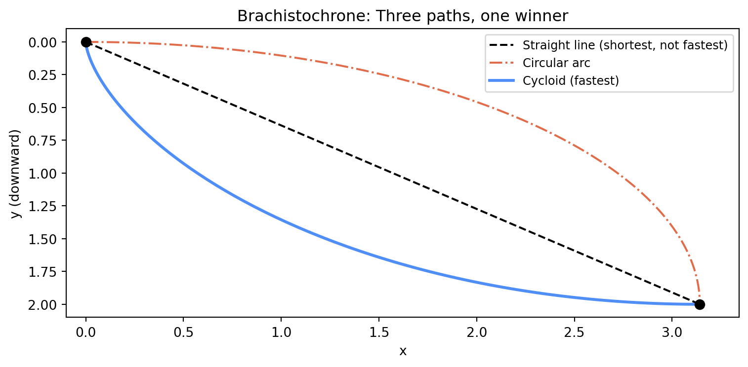
Figure 3.1: Three paths connecting the same two endpoints. The straight line is shortest but not fastest — gravity is not yet fully engaged. The steep initial drop of the cycloid trades height for speed early, winning the race despite covering more distance.

3.4 Why the Cycloid Wins

The cycloid’s initial steep drop is not a coincidence — it is the optimal trade-off between two competing demands. Falling steeply early converts potential energy to kinetic energy quickly, so the bead is moving fast for most of the journey. But too steep an initial drop means the horizontal component of velocity is sacrificed. The cycloid balances these demands exactly.

A physical intuition: Fermat’s principle says light takes the path of least time. When light passes from air into glass, it bends toward the vertical because glass is slower — the light “wants” to spend as little time as possible in the slow medium. The brachistochrone is the same problem in reverse. Gravity plays the role of the refractive index: the bead travels faster at the bottom (where it has fallen further) and slower near the top. The optimal path bends toward the fast region, just as light bends toward the slow region.

Johann Bernoulli’s own solution used exactly this analogy. He applied Snell’s law of refraction to a hypothetical “optical medium” where the refractive index varied with height, and read off the brachistochrone from the path that light would take. It was one of the most elegant solutions in the history of mathematics, and it directly connected optimization to physics in a way that would echo through three centuries of theoretical mechanics.

3.6 The Legacy: Hamilton’s Principle

The most profound application of the Euler-Lagrange equation was Hamilton’s principle of stationary action, published in 1833–1834. William Rowan Hamilton showed that the equations of motion for any mechanical system — Newton’s laws in disguise — could be derived as the Euler-Lagrange equations of a functional, the action:

\[S[q] = \int_{t_1}^{t_2} \mathcal{L}(q, \dot{q}, t)\, dt\]

where $\mathcal{L} = T - V$ is the Lagrangian, the kinetic energy minus the potential energy. Setting $\delta S = 0$ — requiring the action to be stationary — gives the equations of motion.

Hamilton’s principle unified all of Newtonian mechanics under a single variational statement. It later proved to be the foundation of quantum mechanics (Feynman’s path integral) and general relativity (the Einstein-Hilbert action). The brachistochrone problem, which seemed like a mathematical game in 1696, had opened a door that led to the deepest structures in physics.

For optimization, the immediate legacy was a framework for handling infinite-dimensional problems — optimization over spaces of functions — that would eventually develop into optimal control theory. The question “what is the optimal trajectory for a spacecraft?” is a brachistochrone problem dressed in rocket fuel.

3.7 Summary

The brachistochrone problem forced the development of the calculus of variations — a systematic method for finding functions that minimize or maximize integral functionals. The Euler-Lagrange equation is the variational analogue of setting the derivative equal to zero: a necessary condition for optimality. The cycloid is the solution to the brachistochrone problem, and the intuition behind it — exploit fast regions early, match the geometry to the physics — previews the intuition behind every subsequent optimization algorithm.

Hamilton’s reformulation of mechanics as a variational principle revealed that the physical world itself is described by optimization problems. This connection between physics and optimization runs deep enough that Richard Feynman, explaining quantum mechanics to a general audience, used the phrase “nature sniffs out all paths and takes the optimal one.” Whether or not that is literally true, it is a useful way to think.

3.8 Further Reading

Goldstine (1980) covers the brachistochrone and the development of the calculus of variations in full technical detail. For Hamilton’s principle and its consequences, Goldstein, Poole, and Safko’s Classical Mechanics (3rd ed., Addison-Wesley, 2002) is the standard reference. Bernoulli’s original 1696 paper is reproduced in Struik’s A Source Book in Mathematics, 1200–1800 (Princeton, 1969).

--- title: "The Fastest Path" --- ::: {.callout-note} ## Learning Objectives - Understand the brachistochrone problem and its physical setup - Derive the Euler-Lagrange equation for functionals - See how the calculus of variations generalizes derivative-based optimization to function spaces - Understand why the cycloid is the solution and what it implies about optimal paths ::: ## A Challenge Addressed to the World Johann Bernoulli published his brachistochrone problem in January 1696 with the theatrical confidence of a man who knew the answer and suspected very few others did. He was right on both counts. The problem — find the curve of fastest descent for a bead sliding without friction between two points — had exactly five correct solutions submitted within the deadline. All five came from the most formidable mathematicians alive. What made the brachistochrone problem historically significant was not the answer. The cycloid was already known as a curve of elegant properties — Dutch physicist Christiaan Huygens had shown in 1659 that it was also a *tautochrone*, meaning a bead released from any point on a cycloidal arc reaches the bottom in the same time, regardless of starting position. The significance of Bernoulli's challenge was the method required to solve it. Finding the minimum of a function of a real variable requires calculus. Finding the curve that minimizes a time integral requires something more: a calculus of functions, where the unknown is not a number but a curve. The brachistochrone problem forced mathematicians to develop this calculus, and the result — the Euler-Lagrange equation — became one of the most powerful tools in mathematical physics. ## Setting Up the Problem A bead starts at the origin with zero velocity and slides without friction along a wire to a point $(x_1, y_1)$, where $y_1 < 0$ (taking downward as positive $y$). Gravity accelerates the bead downward. What shape should the wire take to minimize the total descent time? The speed of the bead at any height $y$ follows from energy conservation. The kinetic energy gained equals the potential energy lost: $$\frac{1}{2}mv^2 = mgy \implies v = \sqrt{2gy}$$ A small arc length element along the curve $y(x)$ is $ds = \sqrt{1 + (y')^2}\, dx$. The time to traverse this element is $dt = ds/v$. The total descent time is: $$T[y] = \int_0^{x_1} \frac{\sqrt{1 + (y')^2}}{\sqrt{2gy}}\, dx$$ This is a *functional* — a function that takes an entire curve $y(x)$ as its input and returns a real number (the descent time). The brachistochrone problem asks: which function $y(x)$ minimizes $T[y]$? ## The Euler-Lagrange Equation Leonhard Euler, working in the 1740s, developed the systematic method for solving problems of this type. The key insight is to perturb the candidate optimal curve and require that the first-order change in the functional vanish. Let $y^*(x)$ be the optimal curve and let $\eta(x)$ be any smooth function satisfying $\eta(0) = \eta(x_1) = 0$ (the endpoints are fixed). Consider the perturbed curve $y_\epsilon(x) = y^*(x) + \epsilon\, \eta(x)$. The functional becomes $T(\epsilon) = T[y_\epsilon]$, a function of the scalar $\epsilon$. For $y^*$ to be optimal, we need $dT/d\epsilon = 0$ at $\epsilon = 0$. For a general functional $J[y] = \int_a^b F(x, y, y')\, dx$, this condition gives the **Euler-Lagrange equation**: $$\frac{\partial F}{\partial y} - \frac{d}{dx}\frac{\partial F}{\partial y'} = 0$$ This is a necessary condition for an extremum of the functional, exactly analogous to the condition $f'(x) = 0$ for an extremum of an ordinary function. Applied to the brachistochrone functional, where $F = \sqrt{(1+y'^2)/(2gy)}$, it yields a differential equation whose solution is the cycloid. ```{python} #| label: fig-brachistochrone #| fig-cap: "Three paths connecting the same two endpoints. The straight line is shortest but not fastest — gravity is not yet fully engaged. The steep initial drop of the cycloid trades height for speed early, winning the race despite covering more distance." import numpy as np import matplotlib.pyplot as plt def cycloid_path(x1, y1, n=300): """Parametric cycloid from (0,0) to (x1,y1).""" # Find radius R by numerically solving the endpoint condition from scipy.optimize import brentq def endpoint(R): # Parameter theta1 where x(theta1)=x1, y(theta1)=y1 theta_range = np.linspace(0, 2*np.pi, 10000) xs = R*(theta_range - np.sin(theta_range)) ys = R*(1 - np.cos(theta_range)) # Find theta where x closest to x1 idx = np.argmin(np.abs(xs - x1)) return ys[idx] - y1 R = brentq(endpoint, 0.01, 10) theta_range = np.linspace(0, 2*np.pi, n) xs = R*(theta_range - np.sin(theta_range)) ys = R*(1 - np.cos(theta_range)) # Trim to endpoint idx = np.argmin(np.abs(xs - x1)) return xs[:idx+1], ys[:idx+1] x1, y1 = np.pi, 2.0 xc, yc = cycloid_path(x1, y1) fig, ax = plt.subplots(figsize=(8, 4)) # Straight line ax.plot([0, x1], [0, y1], 'k--', linewidth=1.5, label='Straight line (shortest, not fastest)') # Steep initial drop (a circular arc approximation) theta = np.linspace(0, np.pi/2, 200) R_circ = np.sqrt(x1**2 + y1**2) / 2 xr = R_circ * np.sin(theta) * (x1 / (R_circ*np.sin(np.pi/2))) yr = R_circ * (1 - np.cos(theta)) * (y1 / (R_circ*(1-np.cos(np.pi/2)))) ax.plot(xr, yr, color='#e06c4a', linewidth=1.5, linestyle='-.', label='Circular arc') # Cycloid ax.plot(xc, yc, color='#4f8ef7', linewidth=2.2, label='Cycloid (fastest)') ax.scatter([0, x1], [0, y1], s=50, color='k', zorder=5) ax.set_xlabel('x') ax.set_ylabel('y (downward)') ax.set_title('Brachistochrone: Three paths, one winner') ax.legend(fontsize=9) ax.invert_yaxis() ax.set_xlim(-0.1, x1 + 0.2) plt.tight_layout() plt.savefig('figures/brachistochrone.png', dpi=150, bbox_inches='tight') plt.show() ``` ## Why the Cycloid Wins The cycloid's initial steep drop is not a coincidence — it is the optimal trade-off between two competing demands. Falling steeply early converts potential energy to kinetic energy quickly, so the bead is moving fast for most of the journey. But too steep an initial drop means the horizontal component of velocity is sacrificed. The cycloid balances these demands exactly. A physical intuition: Fermat's principle says light takes the path of least time. When light passes from air into glass, it bends toward the vertical because glass is slower — the light "wants" to spend as little time as possible in the slow medium. The brachistochrone is the same problem in reverse. Gravity plays the role of the refractive index: the bead travels faster at the bottom (where it has fallen further) and slower near the top. The optimal path bends toward the fast region, just as light bends toward the slow region. Johann Bernoulli's own solution used exactly this analogy. He applied Snell's law of refraction to a hypothetical "optical medium" where the refractive index varied with height, and read off the brachistochrone from the path that light would take. It was one of the most elegant solutions in the history of mathematics, and it directly connected optimization to physics in a way that would echo through three centuries of theoretical mechanics. ## Lagrange's Refinement Joseph-Louis Lagrange, writing in the 1750s as a teenager in Turin, found a more systematic way to derive the Euler-Lagrange equation and extended it to problems with multiple functions and constraints. His approach — now called the method of Lagrange multipliers — will appear in the next chapter. But his contribution to the calculus of variations was equally important: he showed that the Euler-Lagrange equation is not just a trick for specific problems but a general necessary condition for extrema of functionals. Euler generously renamed the field in Lagrange's honor, calling it the *calculus of variations* (from the Latin for "the calculus of varied curves"), acknowledging that Lagrange's algebraic formulation was cleaner than his own geometric approach. This kind of generosity between mathematicians was characteristic of the eighteenth century and largely disappeared in the nineteenth. ## The Legacy: Hamilton's Principle The most profound application of the Euler-Lagrange equation was Hamilton's principle of stationary action, published in 1833–1834. William Rowan Hamilton showed that the equations of motion for any mechanical system — Newton's laws in disguise — could be derived as the Euler-Lagrange equations of a functional, the *action*: $$S[q] = \int_{t_1}^{t_2} \mathcal{L}(q, \dot{q}, t)\, dt$$ where $\mathcal{L} = T - V$ is the *Lagrangian*, the kinetic energy minus the potential energy. Setting $\delta S = 0$ — requiring the action to be stationary — gives the equations of motion. Hamilton's principle unified all of Newtonian mechanics under a single variational statement. It later proved to be the foundation of quantum mechanics (Feynman's path integral) and general relativity (the Einstein-Hilbert action). The brachistochrone problem, which seemed like a mathematical game in 1696, had opened a door that led to the deepest structures in physics. For optimization, the immediate legacy was a framework for handling infinite-dimensional problems — optimization over spaces of functions — that would eventually develop into optimal control theory. The question "what is the optimal trajectory for a spacecraft?" is a brachistochrone problem dressed in rocket fuel. --- ## Summary The brachistochrone problem forced the development of the calculus of variations — a systematic method for finding functions that minimize or maximize integral functionals. The Euler-Lagrange equation is the variational analogue of setting the derivative equal to zero: a necessary condition for optimality. The cycloid is the solution to the brachistochrone problem, and the intuition behind it — exploit fast regions early, match the geometry to the physics — previews the intuition behind every subsequent optimization algorithm. Hamilton's reformulation of mechanics as a variational principle revealed that the physical world itself is described by optimization problems. This connection between physics and optimization runs deep enough that Richard Feynman, explaining quantum mechanics to a general audience, used the phrase "nature sniffs out all paths and takes the optimal one." Whether or not that is literally true, it is a useful way to think. ## Further Reading @goldstine1980history covers the brachistochrone and the development of the calculus of variations in full technical detail. For Hamilton's principle and its consequences, Goldstein, Poole, and Safko's *Classical Mechanics* (3rd ed., Addison-Wesley, 2002) is the standard reference. Bernoulli's original 1696 paper is reproduced in Struik's *A Source Book in Mathematics, 1200–1800* (Princeton, 1969).