---
title: "The Multiplier"
---
::: {.callout-note}
## Learning Objectives
- Understand Lagrange's method of multipliers for constrained optimization
- Derive the first-order necessary conditions for constrained minima
- Interpret the multiplier as the marginal value of relaxing a constraint
- Connect Lagrange's algebraic approach to modern constrained NLP
:::
## A Mathematician Who Preferred Algebra
Joseph-Louis Lagrange was born in Turin in 1736 to an Italian father and a French mother, spent most of his productive life in Berlin and Paris, and managed to remain on good terms with nearly everyone through the French Revolution — no small achievement. He was the most elegant mathematical writer of his century. Where Euler worked by computation, piling equation upon equation until the answer emerged, Lagrange worked by structure, finding the form that made the result obvious.
His *Mécanique Analytique* of 1788 opens with a declaration of aesthetic principle: "One will not find figures in this work. The methods that I expound require neither constructions nor geometrical or mechanical arguments, but only algebraic operations." Lagrange wanted to strip mechanics of its geometric scaffolding and reduce it to pure calculation. He succeeded so completely that modern mechanics is essentially the *Mécanique Analytique* with updated notation.
The multiplier is Lagrange's most famous contribution to optimization, and its elegance is characteristic: a seemingly artificial trick that, once understood, appears not just useful but inevitable.
## The Problem of Constrained Extrema
Find the maximum of a function $f(x, y)$ subject to the constraint $g(x, y) = 0$.
The naive approach — parametrize the constraint, substitute, and differentiate — works when the constraint is simple but becomes unwieldy for complex constraints or multiple variables. Lagrange's approach replaces the constrained problem with an unconstrained one.
Form the *Lagrangian*:
$$\mathcal{L}(x, y, \lambda) = f(x, y) - \lambda\, g(x, y)$$
The necessary conditions for a stationary point are:
$$\frac{\partial \mathcal{L}}{\partial x} = 0, \quad \frac{\partial \mathcal{L}}{\partial y} = 0, \quad \frac{\partial \mathcal{L}}{\partial \lambda} = 0$$
The third condition recovers the constraint $g(x, y) = 0$. The first two give $\nabla f = \lambda \nabla g$: the gradient of the objective must be parallel to the gradient of the constraint at the solution.
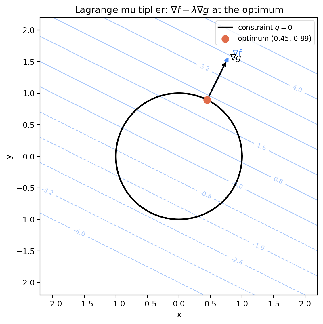
The geometric interpretation is clean: at the constrained optimum, the level curves of $f$ are tangent to the constraint surface. If they were not tangent — if they crossed — you could move along the constraint and increase $f$, contradicting optimality.
```{python}
#| label: fig-lagrange-multiplier
#| fig-cap: "Lagrange multiplier geometry. The optimal point (red dot) is where a level curve of the objective f is tangent to the constraint g = 0. The gradients ∇f and ∇g are parallel there. At any non-optimal feasible point, the gradients are not parallel and movement along the constraint improves the objective."
import numpy as np
import matplotlib.pyplot as plt

fig, ax = plt.subplots(figsize=(7, 6))
x = np.linspace(-2.5, 2.5, 400)
y = np.linspace(-2.5, 2.5, 400)
X, Y = np.meshgrid(x, y)

# Objective: f(x,y) = x + 2y (linear, for clarity)
F = X + 2*Y

# Constraint: x^2 + y^2 = 1 (unit circle)
theta = np.linspace(0, 2*np.pi, 300)
xc = np.cos(theta)
yc = np.sin(theta)

# Optimal point: max of x + 2y on unit circle
# Gradient of f = (1, 2), gradient of g = (2x, 2y)
# At optimum: (1,2) = lambda*(2x, 2y) => x=1/(2lambda), y=1/lambda
# On circle: x^2+y^2=1 => 1/(4l^2)+1/l^2=1 => 5/(4l^2)=1 => l=sqrt(5)/2
# x* = 1/sqrt(5), y* = 2/sqrt(5)
x_opt = 1/np.sqrt(5)
y_opt = 2/np.sqrt(5)

# Level curves of f
levels = np.arange(-4, 5, 0.8)
cs = ax.contour(X, Y, F, levels=levels, colors='#4f8ef7', alpha=0.5, linewidths=1)
ax.clabel(cs, fontsize=8, fmt='%.1f')

# Constraint
ax.plot(xc, yc, 'k-', linewidth=2, label='constraint $g = 0$')

# Optimal point
ax.scatter([x_opt], [y_opt], s=80, color='#e06c4a', zorder=6, label=f'optimum ({x_opt:.2f}, {y_opt:.2f})')

# Gradients at optimal point (scaled for visibility)
scale = 0.35
ax.annotate('', xy=(x_opt + scale*1, y_opt + scale*2),
            xytext=(x_opt, y_opt),
            arrowprops=dict(arrowstyle='->', color='#4f8ef7', lw=1.8))
ax.annotate('', xy=(x_opt + scale*2*x_opt, y_opt + scale*2*y_opt),
            xytext=(x_opt, y_opt),
            arrowprops=dict(arrowstyle='->', color='k', lw=1.8))
ax.text(x_opt + scale*1 + 0.05, y_opt + scale*2, r'$\nabla f$', color='#4f8ef7', fontsize=11)
ax.text(x_opt + scale*2*x_opt + 0.05, y_opt + scale*2*y_opt, r'$\nabla g$', fontsize=11)

ax.set_xlim(-2.2, 2.2)
ax.set_ylim(-2.2, 2.2)
ax.set_aspect('equal')
ax.legend(fontsize=9)
ax.set_title('Lagrange multiplier: $\\nabla f = \\lambda \\nabla g$ at the optimum')
ax.set_xlabel('x')
ax.set_ylabel('y')
plt.tight_layout()
plt.savefig('figures/lagrange_multiplier.png', dpi=150, bbox_inches='tight')
plt.show()
```
## The Multiplier as a Price
The Lagrange multiplier $\lambda$ has a natural economic interpretation that Lagrange himself did not emphasize but that was developed thoroughly by economists in the twentieth century.
Consider a manufacturing firm maximizing profit $f(\mathbf{x})$ subject to a resource constraint $g(\mathbf{x}) = b$ (total resource consumption equals available budget). At the optimum, the multiplier $\lambda^*$ equals $\partial f^*/\partial b$ — the rate of change of maximum profit with respect to the resource budget. It is the *shadow price* of the constraint: how much additional profit the firm could earn if the budget were relaxed by one unit.
This interpretation makes the multiplier concrete. A multiplier near zero means the constraint is not actively limiting — relaxing it would barely help. A large positive multiplier means the constraint is binding tightly — a small relaxation would yield a large gain. In engineering, multipliers on stress constraints tell you which structural member is limiting the design; multipliers on pressure constraints tell you how much performance you are leaving on the table by staying within the operating limit.
## Extending to Inequality Constraints
Lagrange's original formulation handles equality constraints. Engineering problems almost always involve inequality constraints — the chamber pressure must not *exceed* 2,500 psi, not equal it. Extending the multiplier method to inequalities was the work of the twentieth century, and it produced the Kuhn-Tucker conditions discussed in Chapter 7.
The key complication: an inequality constraint $g(\mathbf{x}) \leq 0$ may or may not be active at the optimum. If it is inactive ($g(\mathbf{x}^*) < 0$), it does not constrain the solution and the corresponding multiplier is zero. If it is active ($g(\mathbf{x}^*) = 0$), it acts like an equality constraint with a nonnegative multiplier.
This complementary behavior — either the constraint is active or the multiplier is zero, but not both — is complementary slackness, and it is the heart of modern constrained optimization theory.
## Lagrange in Modern Solvers
Every modern constrained optimization solver — SQP, interior point, augmented Lagrangian — maintains estimates of the Lagrange multipliers alongside the design variables. The multipliers are dual variables; the design variables are primal. Updating both together is what makes these methods efficient.
The augmented Lagrangian method, developed in the 1960s by Hestenes and Powell, adds a penalty term to the Lagrangian to improve conditioning:
$$\mathcal{L}_\rho = f(\mathbf{x}) - \lambda g(\mathbf{x}) + \frac{\rho}{2} g(\mathbf{x})^2$$
The penalty parameter $\rho$ ensures that the augmented Lagrangian is strongly convex near the solution, making it easy to minimize by gradient methods. Iterating between minimizing $\mathcal{L}_\rho$ over $\mathbf{x}$ and updating $\lambda$ produces the alternating direction method of multipliers (ADMM), now one of the dominant algorithms in distributed optimization and machine learning.
---
## Summary
Lagrange's multiplier converts a constrained optimization problem into an unconstrained one by augmenting the objective with a weighted constraint term. The weight — the multiplier — equals the shadow price of the constraint at the optimum: how much the objective would improve if the constraint were relaxed. The geometric condition is tangency: level curves of the objective are tangent to the constraint surface at the solution. Every modern constrained optimization method maintains multiplier estimates and uses them to guide the search.
## Further Reading
@lagrange1788mecanique is the original source. For a modern treatment of multipliers and their economic interpretation, Luenberger's *Linear and Nonlinear Programming* (4th ed., Springer, 2016) is authoritative. Boyd and Vandenberghe's *Convex Optimization* (Cambridge, 2004) covers the augmented Lagrangian and ADMM in depth; the full text is freely available online.