---
title: "The War Problem"
---
::: {.callout-note}
## Learning Objectives
- Understand the wartime origins of linear programming
- Grasp the simplex method geometrically and algorithmically
- Understand why LP became the dominant optimization tool of the twentieth century
- Appreciate Dantzig's role and the institutional context of his discovery
:::
## The Problem of Supplying an Army
In June 1947, a young statistician named George Dantzig walked into the Pentagon with a problem. He had been working for the U.S. Air Force on the question of how to mechanize the planning process — how to take the complex logistical problem of deploying, supplying, and scheduling military forces and turn it into something that could be solved systematically rather than by guesswork and experience.
The core mathematical problem was: minimize a linear function of many variables subject to a system of linear inequality constraints. Dantzig called it linear programming. He did not know at the time that a Soviet economist named Leonid Kantorovich had independently formulated the same problem eight years earlier, or that the mathematical structure had been studied by nineteenth-century French mathematicians in a completely different context. He also did not know that within a decade, the technique he was developing would be used to route every major airline's fleet, schedule every major refinery's production, and plan the supply chains of companies that had not yet been founded.
Dantzig invented the simplex method that summer, working alone. He presented it to the economist John von Neumann in October 1947. Von Neumann listened for a minute, then began pacing and lecturing about duality theory — the mathematical relationship between a linear program and its mirror image — which he had apparently worked out on the spot in the course of the meeting. "I began to feel uneasy," Dantzig wrote later, "in case Johnny was going to work out too much of it before I had a chance to do it myself."
## Linear Programs and Their Geometry
A linear program in standard form minimizes $\mathbf{c}^T \mathbf{x}$ subject to $A\mathbf{x} = \mathbf{b}$, $\mathbf{x} \geq \mathbf{0}$, where $\mathbf{c} \in \mathbb{R}^n$, $A \in \mathbb{R}^{m \times n}$, $\mathbf{b} \in \mathbb{R}^m$.
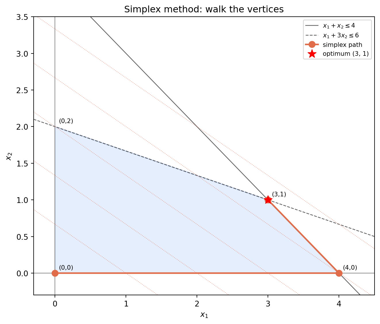
The feasible set is a convex polytope — a many-sided geometric solid. The objective $\mathbf{c}^T\mathbf{x}$ is linear, so its level sets are parallel hyperplanes. The minimum occurs at a vertex of the polytope — a corner point where $n$ constraints are active simultaneously. (It also occurs at a vertex for the maximum, or along an edge if two adjacent vertices achieve the same optimal value.)
This observation is the geometric basis of the simplex method: since the optimum is at a vertex, search only the vertices. Move from vertex to adjacent vertex, improving the objective at each step, until no adjacent vertex is better. Stop.
```{python}
#| label: fig-simplex-geometry
#| fig-cap: "The simplex method in 2D. The feasible polytope (shaded) is bounded by the constraint hyperplanes. The objective contours (dashed parallel lines) move until they are tangent to the polytope. The optimum is at a vertex. The simplex path walks along edges from vertex to vertex, always improving the objective."
import numpy as np
import matplotlib.pyplot as plt
from matplotlib.patches import Polygon
from matplotlib.collections import PatchCollection

fig, ax = plt.subplots(figsize=(7, 6))

# LP: max c^T x, subject to Ax <= b, x >= 0
# max x1 + 1.5*x2
# s.t. x1 + x2 <= 4
#      x1 + 3*x2 <= 6
#      x1, x2 >= 0
# Vertices: (0,0), (4,0), (3,1), (0,2)
vertices = np.array([[0,0],[4,0],[3,1],[0,2]])

poly = Polygon(vertices, closed=True, alpha=0.15, facecolor='#4f8ef7', edgecolor='#2a5ab0', linewidth=1.5)
ax.add_patch(poly)

# Constraint lines
x = np.linspace(-0.3, 4.5, 200)
ax.plot(x, 4 - x, 'k-', linewidth=1, alpha=0.6, label='$x_1 + x_2 \\leq 4$')
ax.plot(x, (6 - x)/3, 'k--', linewidth=1, alpha=0.6, label='$x_1 + 3x_2 \\leq 6$')
ax.axhline(0, color='gray', linewidth=0.8)
ax.axvline(0, color='gray', linewidth=0.8)

# Objective contours: x1 + 1.5*x2 = const
for val in [1, 2, 3, 4, 5]:
    ax.plot(x, (val - x)/1.5, color='#e06c4a', linewidth=0.8, linestyle=':', alpha=0.6)

# Simplex path: (0,0) -> (4,0) -> (3,1)
path = np.array([[0,0],[4,0],[3,1]])
ax.plot(path[:,0], path[:,1], 'o-', color='#e06c4a', linewidth=2, markersize=8, zorder=5, label='simplex path')
ax.scatter([3],[1], s=120, color='red', zorder=6, marker='*', label='optimum (3, 1)')

# Label vertices
for v, lbl in zip(vertices, ['(0,0)','(4,0)','(3,1)','(0,2)']):
    ax.annotate(lbl, v, textcoords='offset points', xytext=(5,5), fontsize=8)

ax.set_xlim(-0.3, 4.5)
ax.set_ylim(-0.3, 3.5)
ax.set_xlabel('$x_1$')
ax.set_ylabel('$x_2$')
ax.set_title('Simplex method: walk the vertices')
ax.legend(fontsize=8, loc='upper right')
plt.tight_layout()
plt.savefig('figures/simplex_geometry.png', dpi=150, bbox_inches='tight')
plt.show()
```
## The Simplex Algorithm
The simplex algorithm is, in its basic form, elegant and simple. Each step:
1. **Current vertex:** maintain a *basic feasible solution* — a vertex of the polytope, identified by a set of $m$ active constraints (basic variables).
2. **Reduced costs:** compute the rate of change of the objective for each non-basic variable. A negative reduced cost (for minimization: positive for a non-basic variable that could increase) indicates that moving in that direction improves the objective.
3. **Pivot:** if any reduced cost indicates improvement, choose one such variable to enter the basis (become active) and another to leave (become inactive). Move to the adjacent vertex.
4. **Optimality:** if no reduced cost indicates improvement, the current vertex is optimal.
The pivot operation is a matrix operation on the basis matrix. In Dantzig's formulation, it is equivalent to a Gaussian elimination step on the constraint matrix. The full algorithm is a sequence of such steps.
## An Exponential Algorithm That Runs in Polynomial Time
The simplex method has an uncomfortable theoretical property: in the worst case, it visits every vertex of the polytope before finding the optimum. The number of vertices can be exponential in the problem dimension — Klee and Minty constructed an explicit example in 1972 where the simplex method visits all $2^n$ vertices of an $n$-dimensional polytope. In theory, the simplex method is exponentially slow.
In practice, it almost never is. The reason is not fully understood. Empirical evidence suggests that the simplex method visits $O(m)$ vertices on typical problems — a number proportional to the number of constraints, not the dimension. Various theoretical explanations have been proposed, involving smoothed analysis (the method is polynomial on randomly perturbed instances) and probabilistic arguments, but none fully explains the observed behavior.
The gap between worst-case and average-case performance is one of the stranger features of the simplex method. It is exponential by construction and polynomial in practice, and the mathematical community spent thirty years after Klee and Minty trying to understand why.
## LP in the World
By 1960, linear programming was being used to plan oil refinery operations, optimize airline crew scheduling, route military supply chains, and manage agricultural production. The problems being solved were large by the standards of the day — thousands of variables and constraints — and required mainframe computers to solve in reasonable time.
The economic impact was enormous. A refinery that runs a daily LP to optimize the allocation of crude oil to products might save several percent of its operating cost. At the scale of a major refinery, that is tens of millions of dollars per year. Airlines solved LP problems to minimize fuel cost, crew hours, and aircraft routing simultaneously. The U.S. military used LP to plan the logistical support of every major operation from Korea through Vietnam.
Dantzig received the National Medal of Science in 1975, the John von Neumann Theory Prize in 1975, and the Harold Pender Award. He did not receive the Nobel Prize. His collaborator Leonid Kantorovich did, in 1975 — the same year.
---
## Summary
Linear programming formulates optimization as minimizing a linear objective over a polytope defined by linear inequalities. The optimum is at a vertex. The simplex method walks from vertex to adjacent vertex, improving the objective at each step, and terminates when no adjacent vertex is better. It is worst-case exponential but average-case polynomial, and it became the dominant optimization tool of the twentieth century within a decade of its invention. George Dantzig invented it in 1947, building on wartime operations research and the emerging theory of linear inequalities.
## Further Reading
@dantzig1963linear is the primary source: Dantzig's own account of the method and its history. @schrijver1998theory provides the mathematical context including Kantorovich's independent work. For the human story, Dantzig's memoir "Linear Programming" in *Operations Research*, 50(1):42–47 (2002), is short and readable.