---
title: "The Modern Toolbox"
---
::: {.callout-note}
## Learning Objectives
- Understand how SQP and trust-region methods handle general NLP
- Understand IPOPT's role in large-scale engineering optimization
- See how algorithmic ideas from different eras combine in modern solvers
- Connect the historical development to the solvers available today
:::
## From Algorithms to Solvers
By 1990, the theoretical foundations of optimization were largely in place. The calculus of variations (Euler, Lagrange, Hamilton) handled infinite-dimensional problems. Linear programming (Dantzig, Kantorovich) handled large linear problems efficiently. The KKT conditions (Karush, Kuhn, Tucker) characterized constrained optima for general smooth NLPs. Interior point methods (Karmarkar and successors) provided polynomial algorithms for LP and, increasingly, NLP. Quasi-Newton methods (Broyden, Fletcher, Goldfarb, Shanno — the BFGS formula of 1970) handled medium-scale unconstrained problems.
What remained was engineering: turning these theoretical algorithms into robust, reliable software that could handle the full range of messy, ill-conditioned, poorly-scaled problems that engineers actually needed to solve.
The 1990s and 2000s were the era of solvers. SNOPT (Gill, Murray, Saunders, 2002) brought SQP to large-scale NLP with a sparse implementation. IPOPT (Wächter and Laird, 2006) brought interior point methods to NLP with the filter line search. KNITRO (Byrd, Nocedal, Waltz) offered both SQP and interior point in a single package. Gurobi and CPLEX dominated LP and mixed-integer LP. These solvers are the tools that engineers actually use, and their development required solving problems that pure mathematical theory did not address: numerical stability, warm starting, infeasibility detection, degenerate problems, and scaling.
## Sequential Quadratic Programming
SQP — the dominant algorithm for medium-scale constrained NLP — builds a quadratic model of the Lagrangian at each iteration and solves a constrained quadratic program (QP) to determine the step direction. The QP subproblem has the same constraints as the original NLP (linearized), which makes the step feasible (or nearly so) by construction.
The key insight, due to Wilson (1963) and Han (1977), is that solving the NLP is equivalent to solving a sequence of QPs, each of which refines the solution. Each QP is fast to solve (quadratic objective, linear constraints), and the sequence converges to the KKT point of the original NLP superlinearly — each iteration roughly squares the error.
SQP's practical advantages: warm-starting (initialize from a nearby previous solution), natural handling of equality constraints, and compatibility with active-set LP solvers for the QP subproblem. Its practical limitation: the QP subproblem requires storing and factoring the Hessian approximation, which costs $O(n^2)$ memory for $n$ variables. For $n > 500$, this becomes impractical on standard hardware.
```{python}
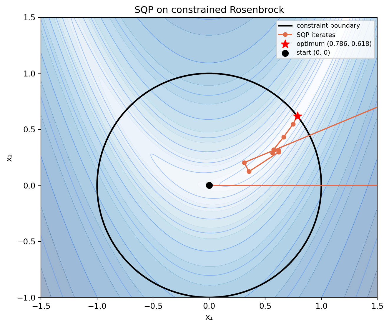
#| label: fig-sqp-convergence
#| fig-cap: "SQP on a constrained NLP: minimize Rosenbrock function subject to a unit disk constraint. Each iteration solves a QP subproblem (shown as the elliptical trust region centered at each iterate). The path converges rapidly to the constrained optimum on the boundary."
import numpy as np
import matplotlib.pyplot as plt
from scipy.optimize import minimize

# Constrained Rosenbrock: min (1-x)^2 + 100(y-x^2)^2
# s.t. x^2 + y^2 <= 1
def rosen(x): return (1-x[0])**2 + 100*(x[1]-x[0]**2)**2
def g(x): return x[0]**2 + x[1]**2 - 1.0  # <= 0

path = [[0., 0.]]
def callback(x): path.append(x.copy())

res = minimize(rosen, [0., 0.], method='SLSQP',
               constraints=[{'type':'ineq', 'fun': lambda x: -g(x)}],
               callback=callback)
path = np.array(path)

fig, ax = plt.subplots(figsize=(7, 6))
x = np.linspace(-1.5, 1.5, 300)
y = np.linspace(-1., 1.5, 300)
X, Y = np.meshgrid(x, y)
Z = np.log1p((1-X)**2 + 100*(Y-X**2)**2)

ax.contourf(X, Y, Z, levels=20, cmap='Blues', alpha=0.4)
ax.contour(X, Y, Z, levels=12, colors='#4f8ef7', alpha=0.5, linewidths=0.7)

theta = np.linspace(0, 2*np.pi, 300)
ax.plot(np.cos(theta), np.sin(theta), 'k-', linewidth=2, label='constraint boundary')

ax.plot(path[:,0], path[:,1], 'o-', color='#e06c4a', markersize=5, linewidth=1.5,
        label='SQP iterates', zorder=4)
ax.scatter(*res.x, s=120, color='red', zorder=6, marker='*', label=f'optimum ({res.x[0]:.3f}, {res.x[1]:.3f})')
ax.scatter(*path[0], s=60, color='k', zorder=5, label='start (0, 0)')

ax.set_xlim(-1.5, 1.5)
ax.set_ylim(-1., 1.5)
ax.set_aspect('equal')
ax.set_xlabel('x₁')
ax.set_ylabel('x₂')
ax.set_title('SQP on constrained Rosenbrock')
ax.legend(fontsize=8)
plt.tight_layout()
plt.savefig('figures/sqp_convergence.png', dpi=150, bbox_inches='tight')
plt.show()
```
## IPOPT and the Filter Line Search
IPOPT (Interior Point OPTimizer), released by Andreas Wächter and Carl Laird in 2006, solved a problem that had blocked practical interior point methods for NLP: globalization.
A pure Newton method applied to the KKT conditions converges quadratically near the solution but can diverge or oscillate from a distant starting point. Globalization — ensuring convergence from any starting point — traditionally used a merit function: a scalar measure combining objective value and constraint violation, monotonically decreased along the search path. The problem is that choosing the weights in the merit function is nontrivial; wrong weights can stall the method near infeasible regions.
Wächter and Laird's filter line search avoids merit function weights entirely. The filter is a list of (objective value, constraint violation) pairs, maintained as a Pareto front. A new iterate is accepted if it dominates at least one entry in the filter — improves either the objective or the constraint violation compared to some prior iterate. The filter prevents cycling without requiring weight tuning.
IPOPT is now the default NLP solver in Julia's JuMP modeling language, the recommended solver for Pyomo in Python, and the solver used by CasADi (a tool widely used in model predictive control and trajectory optimization). It handles problems with hundreds of thousands of variables and sparse Jacobian structures routinely.
## Putting the History Together
The modern constrained NLP solver is a palimpsest of three centuries of mathematical history. The Lagrangian it maintains descends from Lagrange's 1788 multipliers. The KKT conditions it satisfies were derived by Karush in 1939 and Kuhn and Tucker in 1951. The Newton steps it takes descend from Newton's seventeenth-century method. The quasi-Newton Hessian approximation it builds uses the BFGS formula from 1970. The interior point structure traces to Karmarkar's 1984 paper. The filter line search is Wächter and Laird's 2006 contribution.
No single person designed this machine. It assembled itself over centuries, as different mathematicians solved different pieces of a problem they did not fully realize was the same problem. That is usually how it works.
---
## Summary
The modern optimization toolbox — SQP, IPOPT, KNITRO, Gurobi — represents the engineering work of the 1990s and 2000s that turned theoretical algorithms into robust solvers. SQP handles medium-scale NLP through quadratic subproblems, with warm-starting and natural equality constraint handling. IPOPT handles large-scale sparse NLP through interior point methods with filter line search globalization. Each solver embodies decades of accumulated algorithmic ideas from across the history of the field.
## Further Reading
@wachter2006implementation is the IPOPT paper. Gill, Murray, and Saunders' "SNOPT: An SQP algorithm for large-scale constrained optimization" (*SIAM Review*, 47(1):99–131, 2005) describes the dominant SQP solver. @nocedal2006numerical is the comprehensive algorithmic reference for everything in this chapter.