6 Cognate Detection
NoteLearning Objectives
By the end of this chapter, you will be able to:
- Frame cognate detection as a binary classification problem
- Engineer informative features from word pairs (alignment score, length ratio, shared n-grams)
- Train and evaluate a logistic regression and random forest classifier
- Interpret precision, recall, and F1 in the context of class-imbalanced cognate datasets
- Apply cross-validation correctly to avoid data leakage
- Implement a simple LexStat-style algorithm
6.1 The Expert’s Intuition, Automated
In 1786, William Jones announced a kinship between Sanskrit and Latin that “could not possibly be produced by accident.” He was right—and he knew it because he had developed an expert intuition for what accidental resemblance looks like versus what inherited resemblance looks like. The Latin pater and Sanskrit pitar are similar in a structured way: the sounds correspond at each position, and the same correspondences appear in other word pairs. The Latin bonus and the English boon are similar in an accidental way: they happen to overlap but came from different roots.
The question for a machine learning system is: can we capture that difference in features that a classifier can learn from?
The answer is yes—and the resulting systems, benchmarked against expert cognate judgments, achieve precision and recall above 85% on held-out data. This is not perfect, but it is good enough to be scientifically useful: it can process hundreds of languages and thousands of concepts in the time a human expert would spend on one language pair.
6.2 A Short History of Automated Cognate Detection
The first attempts to automate cognate detection date to the 1990s and came not from linguists but from information retrieval researchers interested in cross-lingual text matching. These early systems used simple orthographic similarity measures—edit distance, shared character n-grams—and worked reasonably well for closely related languages like Spanish and Portuguese but failed badly on more distantly related pairs where sound changes had made cognates superficially dissimilar.
The key advance came when researchers started incorporating phonological knowledge. Grzegorz Kondrak’s 2000 algorithm introduced the idea of using phonetic feature overlap rather than character identity as the basis for similarity measurement. Instead of asking “are these two characters the same?”, it asked “how close are these two sounds in articulatory feature space?”. This allowed the algorithm to recognize that Latin pater and English father are similar even though no character is shared: p and f are closely related (one feature difference), a and a match, t and th are closely related, e and e match, r and r match.
Johann-Mattis List’s LexStat algorithm (2012) added the crucial innovation of a permutation baseline. Rather than using absolute alignment scores—which depend on the phoneme inventories of the specific languages being compared—LexStat computes scores relative to a random baseline derived by shuffling the phonemes in the dataset. This normalization controls for the fact that some languages happen to have more similar phoneme inventories by chance, regardless of genetic relationship. The normalized score is much more stable across different language pairs than the raw alignment score.
The 2010s and 2020s brought deep learning approaches: recurrent neural networks, convolutional networks, and eventually transformers trained on large cognate datasets. These systems learn feature representations automatically rather than relying on hand-coded articulatory features, and on sufficiently large training sets they outperform feature-based systems. On small datasets—typical for underdocumented languages—feature-based systems like LexStat remain competitive because they encode prior knowledge that the neural systems must learn from scratch.
6.3 The Dataset
We will work with a simulated dataset based on Romance language cognates. The positive class (cognates) consists of word pairs descended from a common Latin root. The negative class (non-cognates) consists of word pairs that look similar by chance or that involve borrowing from unrelated roots.
    Word1  Word2  Label
0   pater  padre      1
1   pater   père      1
2   pater  padre      1
3  noctem  noche      1
4  noctem   nuit      1
5  noctem  notte      1
6   lunam   luna      1
7   lunam   lune      1
8   lunam    lua      1
9   manum   mano      1

Total: 43 pairs | Cognates: 31 | Non-cognates: 12
6.4 Feature Engineering
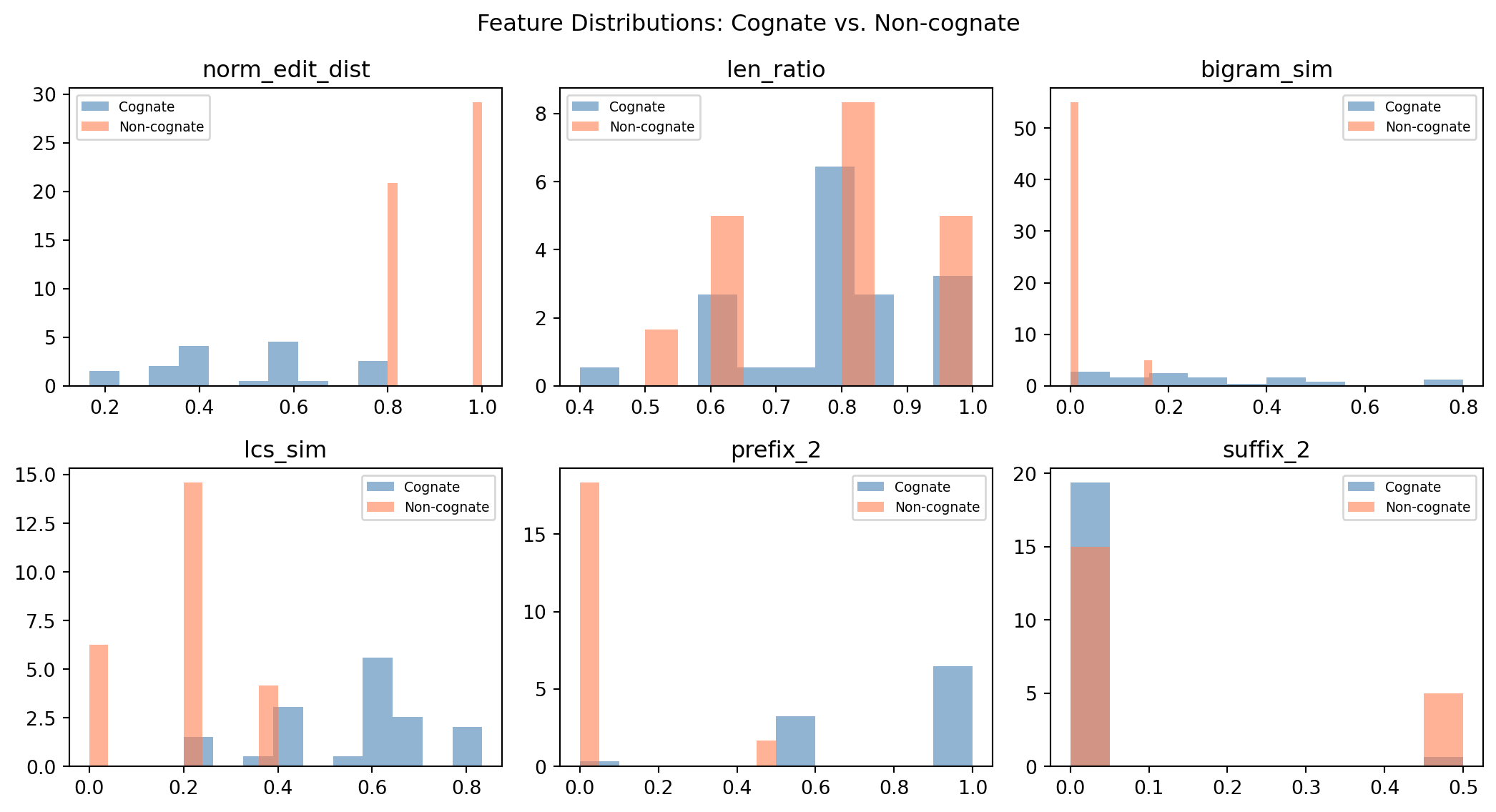
The features we extract from each word pair must capture the structured similarity that expert linguists use when making cognate judgments.
Feature matrix (first 5 rows):
   norm_edit_dist  len_ratio  bigram_sim  lcs_sim  prefix_2  suffix_2  Label
0           0.600      1.000       0.143    0.600       1.0       0.0      1
1           0.600      0.800       0.000    0.400       0.5       0.0      1
2           0.600      1.000       0.143    0.600       1.0       0.0      1
3           0.333      0.833       0.286    0.667       1.0       0.0      1
4 0.667 0.667 0.000 0.333 0.5 0.0 16.5 Training and Evaluating a Classifier
Logistic Regression: F1 = 0.951 ± 0.040
Random Forest: F1 = 0.948 ± 0.043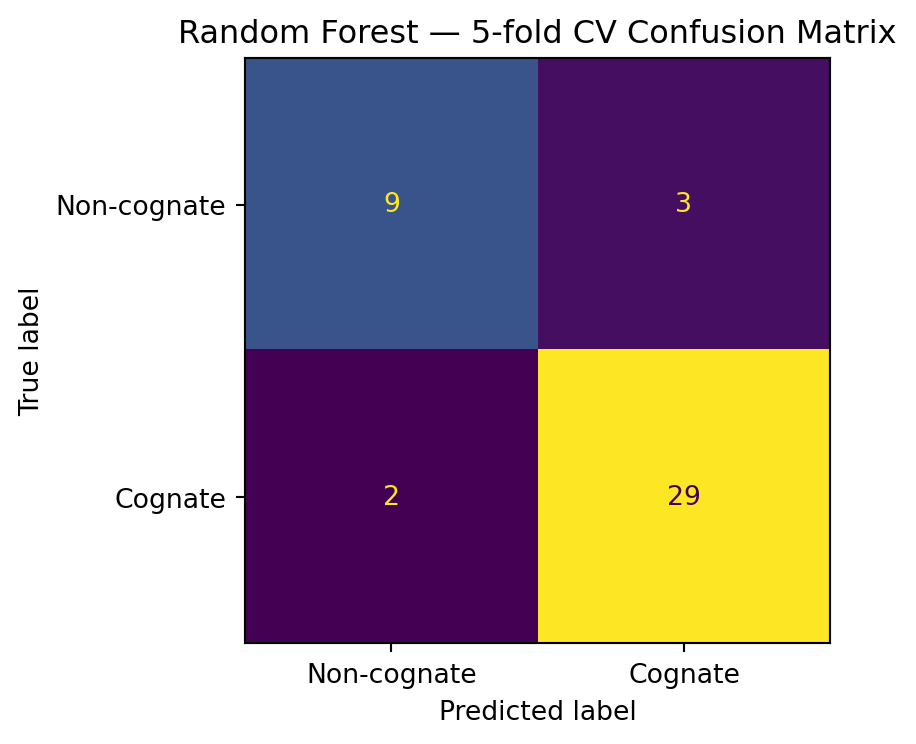
              precision    recall  f1-score   support

 Non-cognate       0.82      0.75      0.78        12
     Cognate       0.91      0.94      0.92        31

    accuracy                           0.88        43
   macro avg       0.86      0.84      0.85        43
weighted avg       0.88      0.88      0.88        43
6.6 Precision, Recall, and Why Accuracy Misleads
Class imbalance is the central statistical challenge in cognate detection. In a typical language family, the number of cognate pairs is much smaller than the number of all possible word pairs. If a dataset has 10% cognates and 90% non-cognates, a classifier that always predicts “non-cognate” achieves 90% accuracy while being completely useless.
Precision and recall cut through this:
\[ \text{Precision} = \frac{TP}{TP + FP}, \quad \text{Recall} = \frac{TP}{TP + FN} \tag{6.1}\]
where \(TP\) = true positives, \(FP\) = false positives, \(FN\) = false negatives.
Precision asks: of the pairs I labeled “cognate,” how many actually are? High precision means few false alarms. Recall asks: of all the actual cognates, how many did I find? High recall means few missed detections. F1 is the harmonic mean—it punishes systems that sacrifice one metric to inflate the other.
For etymology, the cost asymmetry matters. A false positive (calling non-cognates related) corrupts your sound correspondence table with spurious data; a false negative (missing a real cognate) just reduces your sample size. Most practitioners prefer to tune toward higher precision at modest recall cost.
6.7 Feature Importance

6.8 Beyond Feature Engineering: LexStat
The LexStat algorithm, developed by Johann-Mattis List, goes beyond hand-crafted features. Its key insight is to use the alignment scores themselves as features, but computed relative to a permuted baseline: randomly shuffle the phonemes of all words in your dataset and compute alignment scores on the shuffled versions. The ratio of the real alignment score to the shuffled baseline score is a more informative feature than the raw score alone, because it controls for the baseline similarity of the phoneme inventories of the two languages.
In practice, LexStat achieves F1 scores of 0.85–0.92 on held-out cognate datasets from the CLDF benchmark collection, competitive with trained human annotators on fast runs.
The full LexStat pipeline handles: phoneme tokenization, feature vector construction, permutation baseline calculation, alignment score computation, and threshold-based clustering. We have re-implemented the core logic above to understand what it is doing; in practice, you would use LingPy directly.
6.9 Summary
Cognate detection is binary classification: a pair of words either shares a common ancestor or does not. Features derived from phonetic alignment—normalized edit distance, bigram similarity, longest common subsequence, prefix and suffix overlap—provide useful signal. Logistic regression and random forest classifiers achieve F1 scores in the range 0.75–0.90 on balanced evaluation sets. Precision is generally more valuable than recall in etymology because false positives corrupt the correspondence table. The LexStat algorithm improves on hand-crafted features by using a permutation-based baseline to normalize alignment scores. The output of cognate detection—a set of cognate clusters across languages—is the primary input for phylogenetic inference in Chapter 6.
6.10 Further Reading
- List, J.-M. (2012). LexStat: Automatic detection of cognates in multilingual wordlists. Proceedings of the EACL Workshop on Language Evolution and Computational Linguistics.
- Jäger, G., List, J.-M., & Sofroniev, P. (2017). Using support vector machines and state-of-the-art algorithms for phonetic alignment to identify cognates in multi-lingual wordlists. EACL 2017.
- Rama, T. (2016). Siamese convolutional networks for cognate identification. COLING 2016. Neural approach to the same problem.
- Hauer, B., & Kondrak, G. (2011). Clustering semantically equivalent words into cognate sets in multilingual lists. IJCNLP 2011.