Distinguish between the frequentist and Bayesian interpretations of probability
Understand the three axioms of probability and why they constrain belief
Compute conditional probabilities and apply Bayes’ theorem to simple problems
Recognize how prior beliefs influence posterior conclusions
2.1 Two Interpretations of a Simple Number
What does it mean to say there is a 30% chance of rain tomorrow?
The frequentist answers: it means that in a large number of days with atmospheric conditions like today’s, roughly 30% of them were followed by rain. Probability is a property of a class of repeated events. You cannot meaningfully assign a probability to a unique, non-repeatable event — like the outcome of this particular election, or whether a specific patient will survive surgery.
The Bayesian answers differently: a 30% chance of rain is a statement about your state of knowledge. It reflects how confident you are, given everything you know about the current conditions. Probability is not a property of the world; it is a property of the relationship between the world and an observer with incomplete information.
Both interpretations produce the same arithmetic. The difference is philosophical — but philosophy, in this case, has practical consequences that will become apparent when we get to Chapter 3.
2.2 The Axioms and What They Buy You
Whether you are a frequentist or a Bayesian, probability obeys three axioms, stated compactly by Andrey Kolmogorov in 1933:
\(P(A) \geq 0\) for any event \(A\) — probabilities are non-negative.
\(P(\Omega) = 1\) — something in the sample space always happens.
\(P(A \cup B) = P(A) + P(B)\) if \(A\) and \(B\) are mutually exclusive — probabilities of disjoint events add.
These look innocuous. But they have teeth. They imply, for instance, that \(P(A) + P(\neg A) = 1\) — your probability that something happens and your probability that it doesn’t must sum to one. This rules out a certain kind of incoherence: you cannot simultaneously believe there is a 70% chance of rain and a 50% chance of no rain.
A coherent set of beliefs is one that could not be exploited by a clever betting opponent. The Dutch book argument — a classic result in probability theory — shows that anyone whose beliefs violate the axioms can be offered a set of bets that guarantees them a loss regardless of what happens.
2.3 Conditional Probability
Most interesting questions involve conditional probability: given that we know something, how does that change what we expect?
\[P(A \mid B) = \frac{P(A \cap B)}{P(B)} \tag{2.1}\]
Read this as: the probability of \(A\) given \(B\) is the proportion of \(B\)-cases in which \(A\) also occurs. The intuition is simple — conditioning on \(B\) restricts our universe to the subset of events where \(B\) is true, then asks how often \(A\) appears in that subset.
2.4 Bayes’ Theorem: The Arithmetic of Updating
Bayes’ theorem is just a rearrangement of the definition of conditional probability. It is also one of the most useful results in all of science.
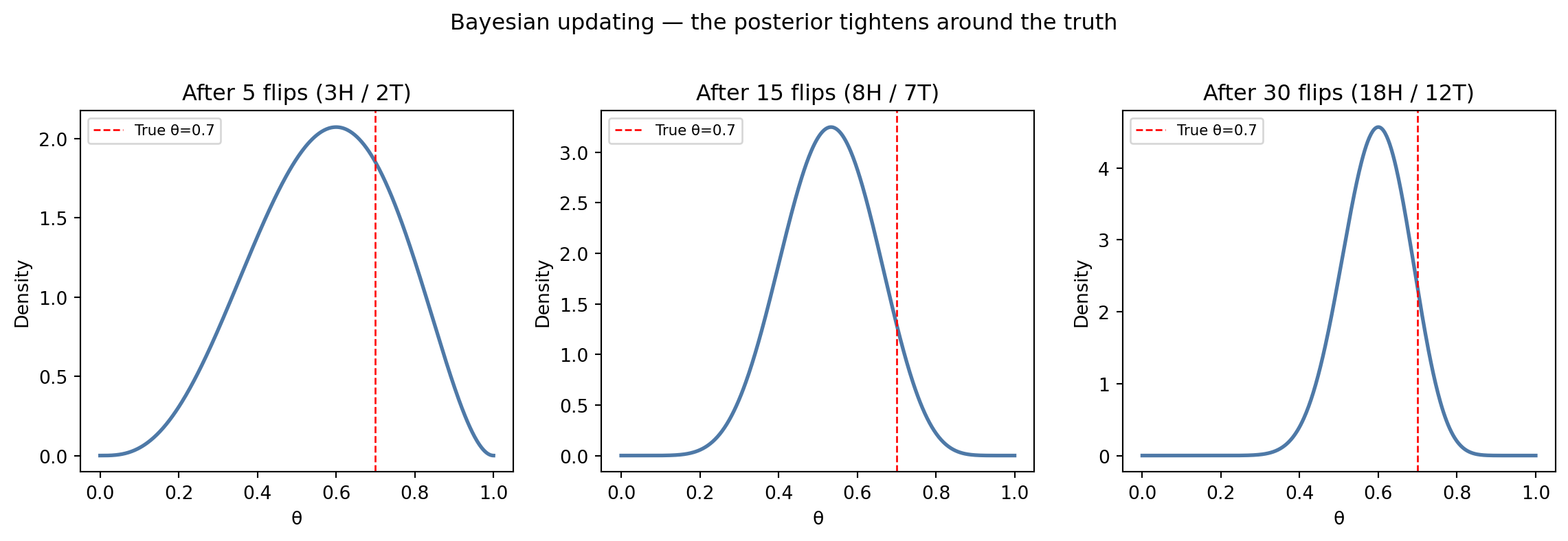
Figure 2.1: Bayesian updating across multiple coin flips. Each observation nudges the posterior toward the true bias.
2.5 Summary
Probability has two main interpretations: frequentist (long-run frequency) and Bayesian (degree of belief). They share the same axioms but answer different questions.
Conditional probability \(P(A \mid B)\) restricts the sample space to cases where \(B\) is true.
Bayes’ theorem is the rule for updating beliefs in response to evidence: prior × likelihood ∝ posterior.
Incoherent beliefs — those that violate the probability axioms — can be exploited by a clever opponent.
2.6 Further Reading
Jaynes (2003) is the definitive case for probability as logic rather than frequency. For a shorter and more accessible treatment, Nate Silver’s The Signal and the Noise covers Bayesian thinking in the real world without heavy mathematics.
Jaynes, Edwin T. 2003. Probability Theory: The Logic of Science. Cambridge University Press.
Source Code
---title: "Probability as Degree of Belief"---::: {.callout-note icon=false}## Learning Objectives- Distinguish between the frequentist and Bayesian interpretations of probability- Understand the three axioms of probability and why they constrain belief- Compute conditional probabilities and apply Bayes' theorem to simple problems- Recognize how prior beliefs influence posterior conclusions:::## Two Interpretations of a Simple NumberWhat does it mean to say there is a 30% chance of rain tomorrow?The frequentist answers: it means that in a large number of days with atmospheric conditions like today's, roughly 30% of them were followed by rain. Probability is a property of a *class of repeated events*. You cannot meaningfully assign a probability to a unique, non-repeatable event — like the outcome of this particular election, or whether a specific patient will survive surgery.The Bayesian answers differently: a 30% chance of rain is a statement about *your state of knowledge*. It reflects how confident you are, given everything you know about the current conditions. Probability is not a property of the world; it is a property of the relationship between the world and an observer with incomplete information.Both interpretations produce the same arithmetic. The difference is philosophical — but philosophy, in this case, has practical consequences that will become apparent when we get to Chapter 3.## The Axioms and What They Buy YouWhether you are a frequentist or a Bayesian, probability obeys three axioms, stated compactly by Andrey Kolmogorov in 1933:1. $P(A) \geq 0$ for any event $A$ — probabilities are non-negative.2. $P(\Omega) = 1$ — something in the sample space always happens.3. $P(A \cup B) = P(A) + P(B)$ if $A$ and $B$ are mutually exclusive — probabilities of disjoint events add.These look innocuous. But they have teeth. They imply, for instance, that $P(A) + P(\neg A) = 1$ — your probability that something happens and your probability that it doesn't must sum to one. This rules out a certain kind of incoherence: you cannot simultaneously believe there is a 70% chance of rain and a 50% chance of no rain.A coherent set of beliefs is one that could not be exploited by a clever betting opponent. The Dutch book argument — a classic result in probability theory — shows that anyone whose beliefs violate the axioms can be offered a set of bets that guarantees them a loss regardless of what happens.## Conditional ProbabilityMost interesting questions involve *conditional* probability: given that we know something, how does that change what we expect?$$P(A \mid B) = \frac{P(A \cap B)}{P(B)}$$ {#eq-conditional}Read this as: the probability of $A$ given $B$ is the proportion of $B$-cases in which $A$ also occurs. The intuition is simple — conditioning on $B$ restricts our universe to the subset of events where $B$ is true, then asks how often $A$ appears in that subset.## Bayes' Theorem: The Arithmetic of UpdatingBayes' theorem is just a rearrangement of the definition of conditional probability. It is also one of the most useful results in all of science.$$P(H \mid D) = \frac{P(D \mid H) \cdot P(H)}{P(D)}$$ {#eq-bayes}Where $H$ is a hypothesis and $D$ is data. In words:- $P(H)$ is the **prior** — your belief in $H$ before seeing $D$.- $P(D \mid H)$ is the **likelihood** — how probable the data would be if $H$ were true.- $P(H \mid D)$ is the **posterior** — your updated belief after seeing $D$.- $P(D)$ is the **marginal likelihood** — a normalizing constant ensuring the posterior sums to one.The theorem tells you, precisely, how much a piece of evidence should change your mind.```{python}#| label: fig-bayes-update#| fig-cap: "Bayesian updating across multiple coin flips. Each observation nudges the posterior toward the true bias."import numpy as npimport matplotlib.pyplot as pltfrom scipy.stats import betarng = np.random.default_rng(42)true_theta =0.7# coin is biased toward headsn_flips =30flips = rng.binomial(1, true_theta, n_flips)theta = np.linspace(0, 1, 500)alpha, b_param =1, 1# start with flat (uniform) priorfig, axes = plt.subplots(1, 3, figsize=(12, 4), sharey=False)checkpoints = [5, 15, 30]for ax, n inzip(axes, checkpoints): heads = flips[:n].sum() tails = n - heads posterior = beta.pdf(theta, alpha + heads, b_param + tails) ax.plot(theta, posterior, color="#4e79a7", linewidth=2) ax.axvline(true_theta, color="red", linestyle="--", linewidth=1, label=f"True θ={true_theta}") ax.set_title(f"After {n} flips ({heads}H / {tails}T)") ax.set_xlabel("θ") ax.set_ylabel("Density") ax.legend(fontsize=8)plt.suptitle("Bayesian updating — the posterior tightens around the truth", y=1.02)plt.tight_layout()plt.show()```## Summary- Probability has two main interpretations: frequentist (long-run frequency) and Bayesian (degree of belief). They share the same axioms but answer different questions.- Conditional probability $P(A \mid B)$ restricts the sample space to cases where $B$ is true.- Bayes' theorem is the rule for updating beliefs in response to evidence: prior × likelihood ∝ posterior.- Incoherent beliefs — those that violate the probability axioms — can be exploited by a clever opponent.## Further Reading@jaynes2003probability is the definitive case for probability as logic rather than frequency. For a shorter and more accessible treatment, Nate Silver's *The Signal and the Noise* covers Bayesian thinking in the real world without heavy mathematics.