Understand why standard ML models cannot answer causal questions
Describe the Double Machine Learning framework for causal effect estimation
Explain causal forests and their advantages over standard random forests
Use DoWhy to estimate a treatment effect from observational data
13.1 The Prediction-Causation Gap
Machine learning is extraordinarily good at prediction. Given a patient’s medical history, it can predict the probability of readmission with striking accuracy. Given a customer’s browsing history, it can predict the probability of purchase. Given atmospheric measurements, it can predict tomorrow’s weather better than any formula a meteorologist could write by hand.
But prediction is Rung 1 on Pearl’s causal ladder. The question “what would happen if we intervened?” is Rung 2, and standard ML models cannot answer it — not because of insufficient data, but because they were not designed to.
A model trained to predict hospital readmissions might learn that patients who receive intensive follow-up care are readmitted less often. Does intensive follow-up cause lower readmission, or are patients receiving intensive follow-up the ones who would have done well anyway? The prediction model cannot tell you. It has absorbed both the causal effect and the selection effect into a single number.
Causal machine learning attempts to answer Rung 2 questions using the tools from both causal inference (Part II) and machine learning (Chapters 11–12).
13.2 Double Machine Learning
Double Machine Learning (Chernozhukov et al., 2018) is an elegant approach to estimating a treatment effect when both the treatment and the outcome depend on high-dimensional covariates.
The key insight: if you want to measure the effect of \(T\) on \(Y\) after accounting for controls \(X\), run two ML models:
Predict \(T\) from \(X\) → get residuals \(\tilde{T} = T - \hat{T}(X)\)
Predict \(Y\) from \(X\) → get residuals \(\tilde{Y} = Y - \hat{Y}(X)\)
Regress \(\tilde{Y}\) on \(\tilde{T}\) → the coefficient is the causal effect estimate
By using residuals — the parts of \(T\) and \(Y\) that the controls cannot explain — you remove the confounding influence of \(X\). The treatment effect estimate is asymptotically normal and valid under weak assumptions on the ML models.
13.3 Causal Forests
A causal forest (Wager and Athey, 2018) estimates heterogeneous treatment effects: not a single average effect, but how the effect varies across individuals.
Standard random forests estimate \(\mathbb{E}[Y \mid X]\). Causal forests estimate \(\tau(x) = \mathbb{E}[Y(1) - Y(0) \mid X = x]\) — the expected treatment effect for an individual with characteristics \(x\).
The construction borrows random forest’s splitting procedure but uses a criterion designed to maximize heterogeneity in treatment effects across leaves, rather than minimizing prediction error.
Code
import numpy as npimport matplotlib.pyplot as plt# Simulate observational data with a confounderrng = np.random.default_rng(42)n =500age = rng.uniform(20, 70, n)# Treatment assignment influenced by age (older → more likely treated)treat_prob =1/ (1+ np.exp(-(age -45) /10))T = rng.binomial(1, treat_prob, n).astype(float)# Outcome: treatment has true effect of 3; age also affects outcomeY =3* T +0.1* age + rng.normal(0, 1, n)# Naive estimate (ignores confounder)naive_ate = Y[T ==1].mean() - Y[T ==0].mean()# Adjusted estimate: regress Y on T and age, read off T coefficientfrom numpy.linalg import lstsqdesign = np.column_stack([T, age, np.ones(n)])coefs, _, _, _ = lstsq(design, Y, rcond=None)adjusted_ate = coefs[0]print(f"True ATE: 3.00")print(f"Naive ATE: {naive_ate:.3f} (biased by confounder)")print(f"Adjusted ATE: {adjusted_ate:.3f} (controls for age)")# Visualizelabels = ["True ATE", "Naive estimate\n(no adjustment)", "Adjusted estimate\n(controls for age)"]values = [3.0, naive_ate, adjusted_ate]colors = ["#59a14f", "#e15759", "#4e79a7"]fig, ax = plt.subplots(figsize=(7, 4))bars = ax.bar(labels, values, color=colors, width=0.5)ax.axhline(3.0, linestyle="--", color="#59a14f", linewidth=1.5, alpha=0.7)ax.set_ylabel("Estimated treatment effect")ax.set_title("Confounder adjustment recovers the true causal effect")for bar, val inzip(bars, values): ax.text(bar.get_x() + bar.get_width()/2, val +0.05, f"{val:.2f}", ha='center', fontsize=10)plt.tight_layout()plt.show()
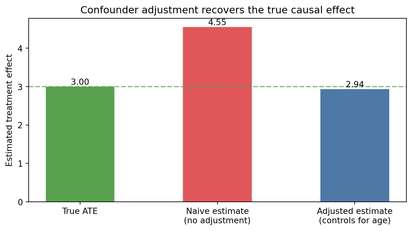
True ATE:     3.00
Naive ATE:    4.554  (biased by confounder)
Adjusted ATE: 2.936  (controls for age)
Figure 13.1: Estimated vs. true average treatment effect using DoWhy on simulated observational data with a measured confounder.
13.4 Summary
Standard ML models optimized for prediction conflate causal effects with selection effects; they cannot answer interventional questions without additional structure.
Double Machine Learning removes the influence of high-dimensional controls from both treatment and outcome before estimating the causal effect, yielding a consistent and asymptotically normal estimator.
Causal forests extend random forests to estimate heterogeneous treatment effects — how the effect of an intervention varies across individuals.
The causal inference framework (DAGs, backdoor criterion, structural models) provides the foundations for all causal ML methods.
13.5 Further Reading
The DoWhy library documentation includes worked examples for each estimation method. Chernozhukov et al. (2018), Double/Debiased Machine Learning for Treatment and Structural Parameters, is the DML reference. Wager and Athey (2018), Estimation and Inference of Heterogeneous Treatment Effects, covers causal forests.
Source Code
---title: "Causal Machine Learning"---::: {.callout-note icon=false}## Learning Objectives- Understand why standard ML models cannot answer causal questions- Describe the Double Machine Learning framework for causal effect estimation- Explain causal forests and their advantages over standard random forests- Use DoWhy to estimate a treatment effect from observational data:::## The Prediction-Causation GapMachine learning is extraordinarily good at prediction. Given a patient's medical history, it can predict the probability of readmission with striking accuracy. Given a customer's browsing history, it can predict the probability of purchase. Given atmospheric measurements, it can predict tomorrow's weather better than any formula a meteorologist could write by hand.But prediction is Rung 1 on Pearl's causal ladder. The question "what would happen if we intervened?" is Rung 2, and standard ML models cannot answer it — not because of insufficient data, but because they were not designed to.A model trained to predict hospital readmissions might learn that patients who receive intensive follow-up care are readmitted less often. Does intensive follow-up *cause* lower readmission, or are patients receiving intensive follow-up the ones who would have done well anyway? The prediction model cannot tell you. It has absorbed both the causal effect and the selection effect into a single number.Causal machine learning attempts to answer Rung 2 questions using the tools from both causal inference (Part II) and machine learning (Chapters 11–12).## Double Machine Learning**Double Machine Learning** (Chernozhukov et al., 2018) is an elegant approach to estimating a treatment effect when both the treatment and the outcome depend on high-dimensional covariates.The key insight: if you want to measure the effect of $T$ on $Y$ after accounting for controls $X$, run two ML models:1. Predict $T$ from $X$ → get residuals $\tilde{T} = T - \hat{T}(X)$2. Predict $Y$ from $X$ → get residuals $\tilde{Y} = Y - \hat{Y}(X)$3. Regress $\tilde{Y}$ on $\tilde{T}$ → the coefficient is the causal effect estimateBy using residuals — the parts of $T$ and $Y$ that the controls cannot explain — you remove the confounding influence of $X$. The treatment effect estimate is asymptotically normal and valid under weak assumptions on the ML models.## Causal ForestsA **causal forest** (Wager and Athey, 2018) estimates *heterogeneous treatment effects*: not a single average effect, but how the effect varies across individuals.Standard random forests estimate $\mathbb{E}[Y \mid X]$. Causal forests estimate $\tau(x) = \mathbb{E}[Y(1) - Y(0) \mid X = x]$ — the expected treatment effect for an individual with characteristics $x$.The construction borrows random forest's splitting procedure but uses a criterion designed to maximize heterogeneity in treatment effects across leaves, rather than minimizing prediction error.```{python}#| label: fig-causal-effect#| fig-cap: "Estimated vs. true average treatment effect using DoWhy on simulated observational data with a measured confounder."import numpy as npimport matplotlib.pyplot as plt# Simulate observational data with a confounderrng = np.random.default_rng(42)n =500age = rng.uniform(20, 70, n)# Treatment assignment influenced by age (older → more likely treated)treat_prob =1/ (1+ np.exp(-(age -45) /10))T = rng.binomial(1, treat_prob, n).astype(float)# Outcome: treatment has true effect of 3; age also affects outcomeY =3* T +0.1* age + rng.normal(0, 1, n)# Naive estimate (ignores confounder)naive_ate = Y[T ==1].mean() - Y[T ==0].mean()# Adjusted estimate: regress Y on T and age, read off T coefficientfrom numpy.linalg import lstsqdesign = np.column_stack([T, age, np.ones(n)])coefs, _, _, _ = lstsq(design, Y, rcond=None)adjusted_ate = coefs[0]print(f"True ATE: 3.00")print(f"Naive ATE: {naive_ate:.3f} (biased by confounder)")print(f"Adjusted ATE: {adjusted_ate:.3f} (controls for age)")# Visualizelabels = ["True ATE", "Naive estimate\n(no adjustment)", "Adjusted estimate\n(controls for age)"]values = [3.0, naive_ate, adjusted_ate]colors = ["#59a14f", "#e15759", "#4e79a7"]fig, ax = plt.subplots(figsize=(7, 4))bars = ax.bar(labels, values, color=colors, width=0.5)ax.axhline(3.0, linestyle="--", color="#59a14f", linewidth=1.5, alpha=0.7)ax.set_ylabel("Estimated treatment effect")ax.set_title("Confounder adjustment recovers the true causal effect")for bar, val inzip(bars, values): ax.text(bar.get_x() + bar.get_width()/2, val +0.05, f"{val:.2f}", ha='center', fontsize=10)plt.tight_layout()plt.show()```## Summary- Standard ML models optimized for prediction conflate causal effects with selection effects; they cannot answer interventional questions without additional structure.- Double Machine Learning removes the influence of high-dimensional controls from both treatment and outcome before estimating the causal effect, yielding a consistent and asymptotically normal estimator.- Causal forests extend random forests to estimate heterogeneous treatment effects — how the effect of an intervention varies across individuals.- The causal inference framework (DAGs, backdoor criterion, structural models) provides the foundations for all causal ML methods.## Further ReadingThe DoWhy library documentation includes worked examples for each estimation method. Chernozhukov et al. (2018), *Double/Debiased Machine Learning for Treatment and Structural Parameters*, is the DML reference. Wager and Athey (2018), *Estimation and Inference of Heterogeneous Treatment Effects*, covers causal forests.