4  Why Correlation Lies

NoteLearning Objectives

• Understand Simpson’s Paradox and why aggregated data can reverse a trend
• Define confounders and colliders and explain why they distort associations
• Recognize the structural reasons that correlation does not imply causation
• Compute and visualize a Simpson’s Paradox example in Python

4.1 A Tale Told Backwards

In 1973, UC Berkeley was sued for gender bias in graduate admissions. The data seemed damning: of 8,442 men who applied, 44% were admitted; of 4,321 women, only 35% were admitted. When researchers looked more carefully, however, something unexpected emerged. When they broke the data down by department, women were admitted at a higher rate than men in most departments. The aggregated statistic had reversed the truth.

This is Simpson’s Paradox: a trend that appears in several groups of data can disappear — or reverse — when those groups are combined. The reason, in Berkeley’s case, was a lurking variable: women disproportionately applied to highly competitive departments with low acceptance rates for everyone. The overall admission rate reflected departmental selectivity, not gender discrimination.

Simpson’s Paradox is not a quirk. It is a warning label on every dataset you will ever analyze.

4.2 Confounders and Colliders

A confounder is a variable that influences both the cause and the effect we are studying, creating a spurious association between them. If we observe that shoe size correlates with reading ability in children, the confounder is age: older children have larger feet and read better. Shoe size does not cause literacy.

A collider is more subtle. It is a variable that is caused by two other variables, and conditioning on it can create a spurious association between its causes. If both talent and luck determine whether someone becomes famous, then among famous people, talent and luck are negatively correlated — you needed one if you lacked the other. Conditioning on fame (the collider) introduces a relationship that does not exist in the general population.

Understanding the difference between confounders and colliders is the difference between adjusting for the right variables and adjusting for the wrong ones. Statistical practice has long recommended “controlling for everything.” Causal theory shows that this advice can actively mislead you.

4.3 The Structural Picture

Consider a simple scenario: ice cream sales and drowning deaths are correlated. The confounder is hot weather, which causes both. If you naively regress drowning deaths on ice cream sales, you will find a positive relationship. Intervening on ice cream sales — shutting every ice cream truck in the country — would not reduce drowning deaths.

The association exists. The causal relationship does not. No amount of statistical sophistication can recover the distinction without additional structural assumptions — assumptions about how the data was generated.

This is the central insight that motivates Part II of this book.

import numpy as np
import matplotlib.pyplot as plt

rng = np.random.default_rng(0)

# Three groups with different (x, y) offsets — each has positive slope
groups = [(1, 5), (4, 3), (7, 1)]   # (x_offset, y_offset)
colors = ["#4e79a7", "#f28e2b", "#59a14f"]
all_x, all_y = [], []

fig, ax = plt.subplots(figsize=(8, 5))

for (xo, yo), col in zip(groups, colors):
    x = rng.uniform(0, 2, 30) + xo
    y = 0.5 * x + rng.normal(0, 0.3, 30) + yo - 0.5 * xo
    ax.scatter(x, y, color=col, alpha=0.6, s=30)
    m = np.polyfit(x, y, 1)
    xs = np.linspace(x.min(), x.max(), 100)
    ax.plot(xs, np.polyval(m, xs), color=col, linewidth=2)
    all_x.extend(x); all_y.extend(y)

# Overall (spurious) trend
all_x, all_y = np.array(all_x), np.array(all_y)
m_all = np.polyfit(all_x, all_y, 1)
xs_all = np.linspace(all_x.min(), all_x.max(), 300)
ax.plot(xs_all, np.polyval(m_all, xs_all), color="gray", linewidth=2.5,
        linestyle="--", label="Overall trend (misleading)")
ax.set_xlabel("X"); ax.set_ylabel("Y")
ax.set_title("Simpson's Paradox")
ax.legend()
plt.tight_layout()
plt.show()

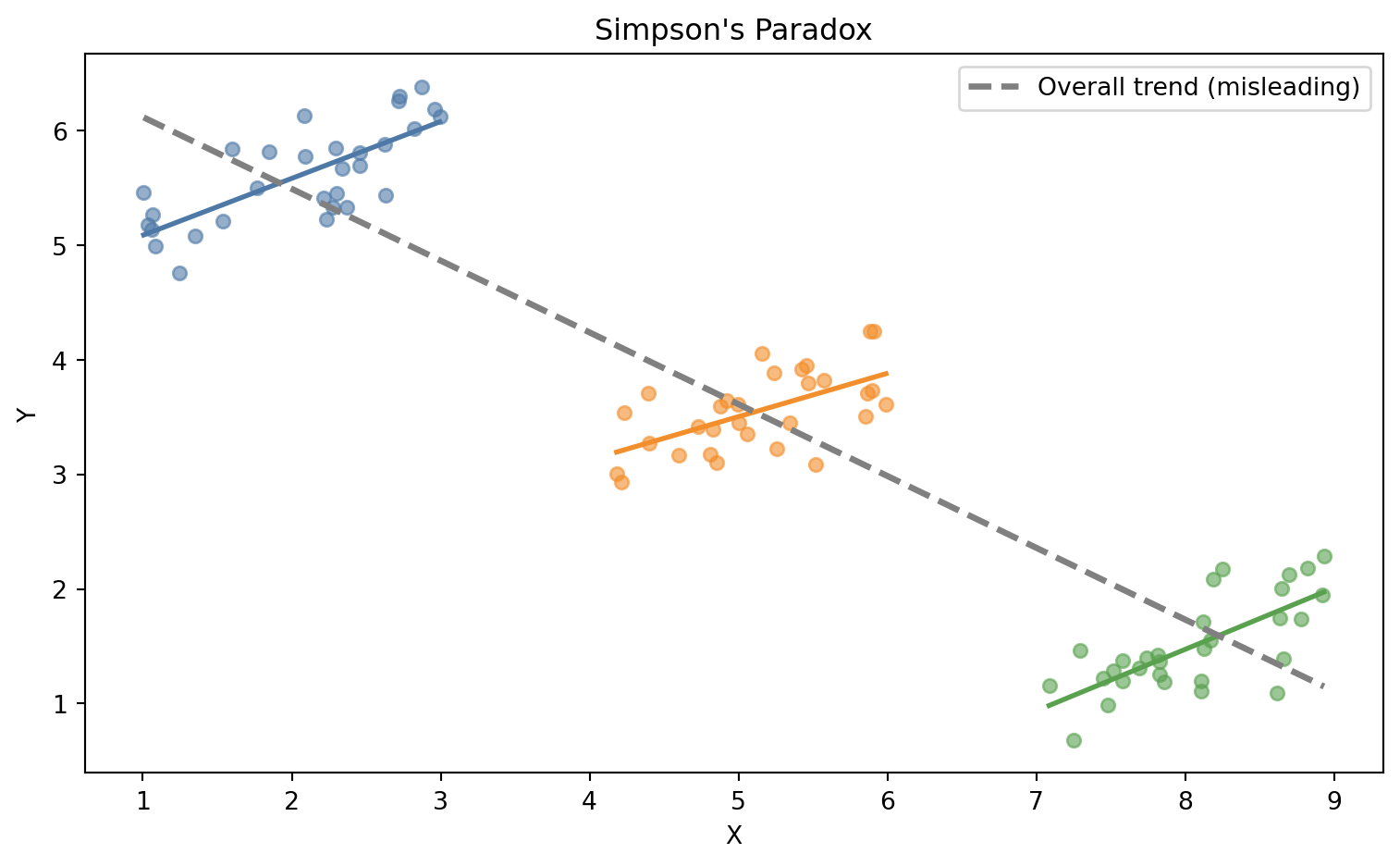
Figure 4.1: Simpson’s Paradox: the overall trend (gray) suggests a negative relationship. Within each group (colored), the trend is positive.

4.4 Summary

• Simpson’s Paradox shows that aggregating data across groups can reverse the direction of an association.
• Confounders are variables that cause both the treatment and the outcome, creating spurious associations.
• Colliders are variables caused by two others; conditioning on a collider introduces spurious associations between its causes.
• Statistical correlation, however carefully measured, cannot distinguish causal relationships from artifacts of the data-generating process.

4.5 Further Reading

Pearl and Mackenzie (2018) opens with an extended discussion of Simpson’s Paradox that is more accessible than any academic treatment. Judea Pearl’s original technical work on confounders and colliders is in Pearl (2009), which is thorough but requires patience.

Pearl, Judea. 2009. Causality: Models, Reasoning, and Inference. 2nd ed. Cambridge University Press.

Pearl, Judea, and Dana Mackenzie. 2018. The Book of Why: The New Science of Cause and Effect. Basic Books.