Understand linear and logistic regression as optimization problems
Trace the conceptual path from the perceptron to multi-layer networks
Understand what a neural network is learning and why depth matters
Train a small neural network using scikit-learn and interpret the result
11.1 The Simplest Learner
Linear regression is one of the oldest and most useful ideas in statistics. Given a set of inputs \(\mathbf{x}\) and a numerical output \(y\), it finds a weighted combination of the inputs that best predicts the output:
The weights \(\mathbf{w}\) are chosen to minimize the mean squared error over the training data. The result is a linear model: the prediction surface is a hyperplane.
This simplicity is both the strength and the limitation of linear regression. It makes the model interpretable — each weight tells you, directly, how much a unit increase in \(x_i\) shifts the prediction. But it cannot capture non-linear relationships. A system that behaves like a parabola, or a sinusoid, or an interaction between two variables, will not be well-served by a linear model.
11.2 Logistic Regression and the Classification Problem
When the output is a category rather than a continuous number, we need a different approach. Logistic regression models the probability of belonging to a class:
The sigmoid function \(\sigma\) squashes any real number into \((0, 1)\), making it interpretable as a probability. Despite the name, logistic “regression” is a classifier. The decision boundary is a hyperplane.
11.3 The Perceptron and Its Limits
Frank Rosenblatt’s perceptron (1958) was an early attempt to build a learning machine modeled loosely on the neuron. It is essentially a logistic regression with a step activation instead of sigmoid: output 1 if the weighted sum exceeds a threshold, 0 otherwise.
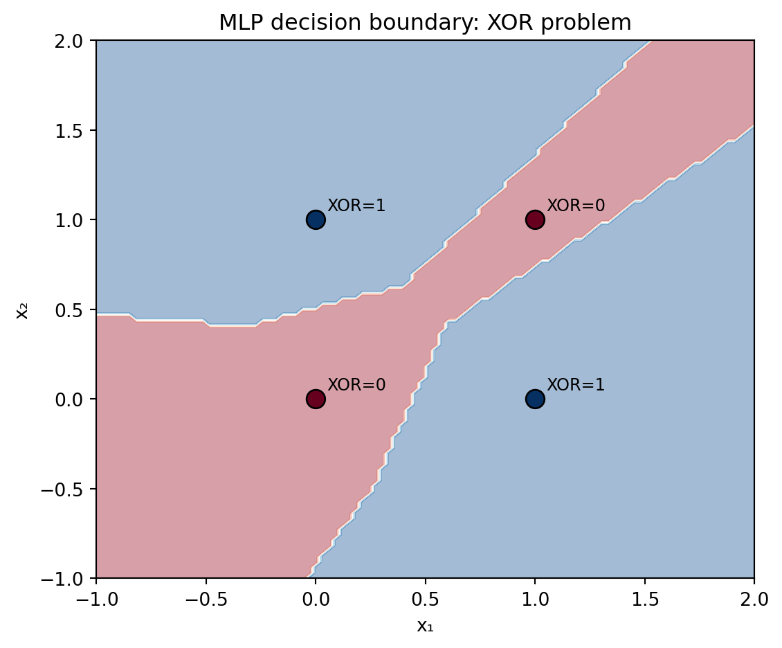
The perceptron can learn any linearly separable classification problem. In 1969, Minsky and Papert proved that it cannot learn XOR — a pattern that requires a non-linear boundary. This result temporarily deflated enthusiasm for neural networks.
The fix, which took another decade to fully materialize, was to stack perceptrons in layers.
11.4 Multi-Layer Networks
A multi-layer network adds one or more hidden layers between input and output. Each hidden unit computes a weighted sum of its inputs and applies a non-linear activation function. This breaks the linearity constraint.
The key insight: a single hidden layer with enough units can approximate any continuous function to arbitrary accuracy (the Universal Approximation Theorem). Multiple layers allow the network to learn hierarchical representations — each layer building on the features learned by the layer below.
Training is done by backpropagation: compute the gradient of the loss with respect to every weight in the network, then update the weights in the direction that reduces the loss.
Figure 11.1: A multi-layer network learns the non-linear XOR boundary that a single perceptron cannot. Decision regions shown.
11.5 Summary
Linear regression finds the best-fitting hyperplane through the data; it is interpretable but cannot capture non-linear patterns.
Logistic regression extends linear regression to classification by applying the sigmoid function.
The perceptron learns linearly separable problems; the multi-layer network overcomes this limitation through hidden layers and non-linear activations.
Backpropagation computes gradients efficiently by applying the chain rule through the network; it is the engine of modern deep learning.
11.6 Further Reading
Goodfellow et al. (2016) is the standard graduate-level reference. Chapter 6 covers multi-layer networks in depth. For a more accessible treatment, Michael Nielsen’s free online book Neural Networks and Deep Learning (neuralnetworksanddeeplearning.com) is excellent.
Goodfellow, Ian, Yoshua Bengio, and Aaron Courville. 2016. Deep Learning. MIT Press.
Source Code
---title: "From Regression to Neural Networks"---::: {.callout-note icon=false}## Learning Objectives- Understand linear and logistic regression as optimization problems- Trace the conceptual path from the perceptron to multi-layer networks- Understand what a neural network is learning and why depth matters- Train a small neural network using scikit-learn and interpret the result:::## The Simplest LearnerLinear regression is one of the oldest and most useful ideas in statistics. Given a set of inputs $\mathbf{x}$ and a numerical output $y$, it finds a weighted combination of the inputs that best predicts the output:$$\hat{y} = w_0 + w_1 x_1 + w_2 x_2 + \ldots + w_p x_p$$ {#eq-linear-reg}The weights $\mathbf{w}$ are chosen to minimize the mean squared error over the training data. The result is a *linear model*: the prediction surface is a hyperplane.This simplicity is both the strength and the limitation of linear regression. It makes the model interpretable — each weight tells you, directly, how much a unit increase in $x_i$ shifts the prediction. But it cannot capture non-linear relationships. A system that behaves like a parabola, or a sinusoid, or an interaction between two variables, will not be well-served by a linear model.## Logistic Regression and the Classification ProblemWhen the output is a category rather than a continuous number, we need a different approach. Logistic regression models the *probability* of belonging to a class:$$P(y = 1 \mid \mathbf{x}) = \sigma(\mathbf{w}^T \mathbf{x}) = \frac{1}{1 + e^{-\mathbf{w}^T \mathbf{x}}}$$ {#eq-logistic}The sigmoid function $\sigma$ squashes any real number into $(0, 1)$, making it interpretable as a probability. Despite the name, logistic "regression" is a classifier. The decision boundary is a hyperplane.## The Perceptron and Its LimitsFrank Rosenblatt's perceptron (1958) was an early attempt to build a learning machine modeled loosely on the neuron. It is essentially a logistic regression with a step activation instead of sigmoid: output 1 if the weighted sum exceeds a threshold, 0 otherwise.The perceptron can learn any *linearly separable* classification problem. In 1969, Minsky and Papert proved that it cannot learn XOR — a pattern that requires a non-linear boundary. This result temporarily deflated enthusiasm for neural networks.The fix, which took another decade to fully materialize, was to stack perceptrons in layers.## Multi-Layer NetworksA multi-layer network adds one or more *hidden layers* between input and output. Each hidden unit computes a weighted sum of its inputs and applies a non-linear activation function. This breaks the linearity constraint.The key insight: a single hidden layer with enough units can approximate *any* continuous function to arbitrary accuracy (the Universal Approximation Theorem). Multiple layers allow the network to learn hierarchical representations — each layer building on the features learned by the layer below.Training is done by backpropagation: compute the gradient of the loss with respect to every weight in the network, then update the weights in the direction that reduces the loss.```{python}#| label: fig-mlp-nonlinear#| fig-cap: "A multi-layer network learns the non-linear XOR boundary that a single perceptron cannot. Decision regions shown."import numpy as npimport matplotlib.pyplot as pltfrom sklearn.neural_network import MLPClassifierfrom sklearn.inspection import DecisionBoundaryDisplay# XOR dataX = np.array([[0,0],[0,1],[1,0],[1,1]])y = np.array([0, 1, 1, 0])clf = MLPClassifier(hidden_layer_sizes=(8, 8), activation='relu', max_iter=2000, random_state=0)clf.fit(X, y)fig, ax = plt.subplots(figsize=(6, 5))disp = DecisionBoundaryDisplay.from_estimator(clf, X, response_method="predict", ax=ax, alpha=0.4, cmap=plt.cm.RdBu)ax.scatter(X[:, 0], X[:, 1], c=y, cmap=plt.cm.RdBu, edgecolors='k', s=100, zorder=5)for xi, label inzip(X, y): ax.annotate(f"XOR={label}", (xi[0]+0.05, xi[1]+0.05), fontsize=9)ax.set_title("MLP decision boundary: XOR problem")ax.set_xlabel("x₁"); ax.set_ylabel("x₂")plt.tight_layout()plt.show()```## Summary- Linear regression finds the best-fitting hyperplane through the data; it is interpretable but cannot capture non-linear patterns.- Logistic regression extends linear regression to classification by applying the sigmoid function.- The perceptron learns linearly separable problems; the multi-layer network overcomes this limitation through hidden layers and non-linear activations.- Backpropagation computes gradients efficiently by applying the chain rule through the network; it is the engine of modern deep learning.## Further Reading@goodfellow2016deep is the standard graduate-level reference. Chapter 6 covers multi-layer networks in depth. For a more accessible treatment, Michael Nielsen's free online book *Neural Networks and Deep Learning* (neuralnetworksanddeeplearning.com) is excellent.