This appendix collects the mathematical background assumed throughout the book. Readers with a strong quantitative background can skip it. Those encountering some topics for the first time may find it useful to work through the relevant sections before or alongside the corresponding chapters.
Probability Theory
Random variables. A random variable \(X\) is a function from a sample space to the real numbers. Its distribution describes the probability of each possible value.
Expectation. The expected value \(\mathbb{E}[X] = \sum_x x \cdot P(X = x)\) (discrete) or \(\int x \cdot f(x) \, dx\) (continuous).
Variance. \(\text{Var}(X) = \mathbb{E}[(X - \mathbb{E}[X])^2] = \mathbb{E}[X^2] - (\mathbb{E}[X])^2\).
Conditional independence. \(X \perp Y \mid Z\) means that, given \(Z\), knowing \(X\) provides no additional information about \(Y\): \(P(X \mid Y, Z) = P(X \mid Z)\).
Bayes’ theorem. \(P(H \mid D) = P(D \mid H) P(H) / P(D)\).
Common distributions used in this book:
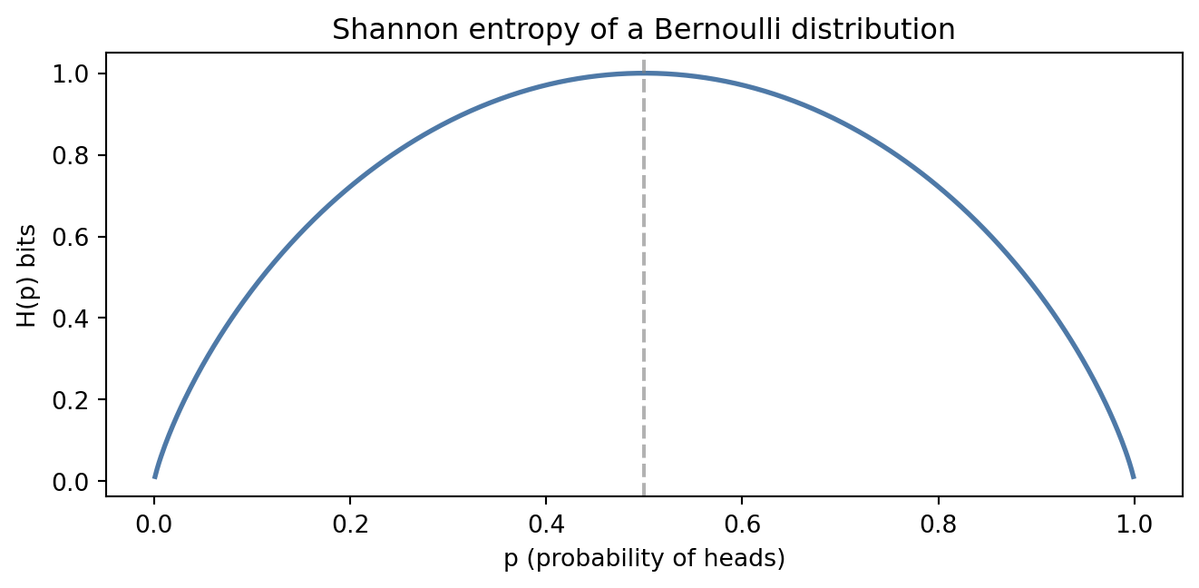
| Bernoulli |
\(p\) |
\(\{0, 1\}\) |
Binary outcomes |
| Binomial |
\(n, p\) |
\(\{0, \ldots, n\}\) |
Count of successes |
| Beta |
\(\alpha, \beta\) |
\([0, 1]\) |
Prior on probabilities |
| Normal |
\(\mu, \sigma^2\) |
\(\mathbb{R}\) |
Continuous data, errors |
| Gamma |
\(\alpha, \beta\) |
\((0, \infty)\) |
Positive quantities, rates |
| Poisson |
\(\lambda\) |
\(\{0, 1, 2, \ldots\}\) |
Count data |
Linear Algebra Basics
Vectors. A column vector \(\mathbf{x} \in \mathbb{R}^n\) is a list of \(n\) numbers.
Dot product. \(\mathbf{a} \cdot \mathbf{b} = \sum_i a_i b_i\). Geometrically, \(\mathbf{a} \cdot \mathbf{b} = \|\mathbf{a}\| \|\mathbf{b}\| \cos\theta\).
Matrix multiplication. \((AB)_{ij} = \sum_k A_{ik} B_{kj}\).
Transpose. \((A^T)_{ij} = A_{ji}\).
The notation \(\mathbf{w}^T \mathbf{x}\) denotes the dot product of two column vectors — used throughout for linear models.
Calculus Notation
Derivative. \(f'(x) = \frac{df}{dx}\): rate of change of \(f\) with respect to \(x\).
Partial derivative. \(\frac{\partial f}{\partial x_i}\): rate of change of \(f\) with respect to \(x_i\), holding all other variables constant.
Gradient. \(\nabla_\theta f = \left(\frac{\partial f}{\partial \theta_1}, \ldots, \frac{\partial f}{\partial \theta_n}\right)^T\): vector of all partial derivatives.
Chain rule. If \(z = f(g(x))\), then \(\frac{dz}{dx} = \frac{dz}{dg} \cdot \frac{dg}{dx}\). This is the backbone of backpropagation.
Integral. \(\int_a^b f(x) \, dx\): area under the curve \(f\) from \(a\) to \(b\).