---
title: "Reinforcement Learning"
---
::: {.callout-note icon=false}
## Learning Objectives
- Describe the reinforcement learning framework: agents, states, actions, rewards
- Formalize the problem as a Markov Decision Process (MDP)
- Understand the Q-learning algorithm and why it works
- Implement Q-learning on a simple grid-world environment
:::
## Learning by Doing
All of the learning frameworks we have seen so far are *passive*: the learner receives data and updates its beliefs or its model parameters. The data is simply there, handed over.
Reinforcement learning is different. The agent exists in an environment. It takes actions. Those actions change the environment's state. The environment responds with a reward signal — positive for good outcomes, negative for bad ones. The agent's goal is to learn a policy: a mapping from states to actions that maximizes the expected cumulative reward over time.
This is the learning structure most recognizable from biology. A rat in a maze learns not from a textbook but from running the maze, getting cheese, finding dead ends, and gradually building a map of what works. A child learns to walk through exactly this process — try, fall, try again, receive the reward of not falling.
What makes reinforcement learning computationally interesting is the *credit assignment problem*: if an agent receives a reward after a long sequence of actions, which of those actions was responsible for it? The action taken three steps ago may have been the critical one, not the last action.
## Markov Decision Processes
A Markov Decision Process (MDP) is the formal framework for RL problems:
- $\mathcal{S}$: set of states
- $\mathcal{A}$: set of actions
- $P(s' \mid s, a)$: transition probability — given state $s$ and action $a$, what is the probability of landing in state $s'$?
- $R(s, a, s')$: reward received when transitioning from $s$ to $s'$ via action $a$
- $\gamma \in [0, 1)$: discount factor — future rewards are worth less than immediate rewards
The agent's goal is to find a policy $\pi(a \mid s)$ that maximizes the expected discounted return:
$$G_t = \sum_{k=0}^{\infty} \gamma^k R_{t+k+1}$$ {#eq-return}
## Q-Learning
Q-learning (Watkins, 1989) is a model-free algorithm: the agent does not need to know the transition probabilities $P(s' \mid s, a)$. Instead, it learns a **Q-function**: the expected cumulative reward from taking action $a$ in state $s$ and then following the optimal policy thereafter.
The Q-function is updated from experience using the Bellman equation:
$$Q(s, a) \leftarrow Q(s, a) + \alpha \left[ r + \gamma \max_{a'} Q(s', a') - Q(s, a) \right]$$ {#eq-q-update}
The term in brackets is the **temporal difference error** — the difference between the estimated value and the new estimate based on the observed reward and the next state's value. With enough experience, $Q$ converges to the optimal Q-function, and the optimal policy is simply to always take the action with the highest Q-value.
```{python}
#| label: fig-gridworld
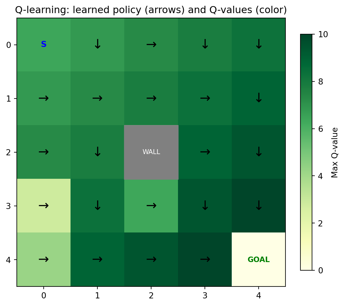
#| fig-cap: "Q-learning on a 5×5 grid world. The agent learns to navigate from start (top-left) to goal (bottom-right) while avoiding the obstacle."
import numpy as np
import matplotlib.pyplot as plt
import matplotlib.patches as mpatches

# 5x5 grid world
# States: (row, col) flattened to index
# Actions: 0=up, 1=down, 2=left, 3=right
GRID = 5
GOAL = (4, 4)
OBSTACLE = (2, 2)
START = (0, 0)

def state_idx(r, c): return r * GRID + c

def step(state, action):
    r, c = divmod(state, GRID)
    dr, dc = [(-1,0),(1,0),(0,-1),(0,1)][action]
    nr, nc = max(0, min(GRID-1, r+dr)), max(0, min(GRID-1, c+dc))
    if (nr, nc) == OBSTACLE:
        nr, nc = r, c  # blocked
    next_state = state_idx(nr, nc)
    reward = 10.0 if (nr, nc) == GOAL else -0.1
    done = (nr, nc) == GOAL
    return next_state, reward, done

rng = np.random.default_rng(0)
Q = np.zeros((GRID*GRID, 4))
alpha, gamma, episodes = 0.1, 0.95, 3000
epsilon = 0.3

for ep in range(episodes):
    s = state_idx(*START)
    for _ in range(200):
        if rng.random() < epsilon:
            a = rng.integers(4)
        else:
            a = int(np.argmax(Q[s]))
        ns, r, done = step(s, a)
        Q[s, a] += alpha * (r + gamma * np.max(Q[ns]) - Q[s, a])
        s = ns
        if done:
            break
    epsilon = max(0.05, epsilon * 0.999)

# Extract greedy policy
policy_arrows = {0: '↑', 1: '↓', 2: '←', 3: '→'}
grid_policy = np.argmax(Q, axis=1).reshape(GRID, GRID)

fig, ax = plt.subplots(figsize=(6, 6))
value_grid = np.max(Q, axis=1).reshape(GRID, GRID)
im = ax.imshow(value_grid, cmap='YlGn', vmin=0)
plt.colorbar(im, ax=ax, fraction=0.04, label="Max Q-value")

for r in range(GRID):
    for c in range(GRID):
        if (r, c) == GOAL:
            ax.text(c, r, 'GOAL', ha='center', va='center', fontsize=9, fontweight='bold', color='green')
        elif (r, c) == OBSTACLE:
            ax.add_patch(mpatches.Rectangle((c-0.5, r-0.5), 1, 1, color='gray'))
            ax.text(c, r, 'WALL', ha='center', va='center', fontsize=8, color='white')
        elif (r, c) == START:
            ax.text(c, r, 'S', ha='center', va='center', fontsize=10, fontweight='bold', color='blue')
        else:
            ax.text(c, r, policy_arrows[grid_policy[r, c]],
                    ha='center', va='center', fontsize=16)

ax.set_title("Q-learning: learned policy (arrows) and Q-values (color)")
ax.set_xticks(range(GRID)); ax.set_yticks(range(GRID))
plt.tight_layout()
plt.show()
```
## Summary
- Reinforcement learning is the framework for learning through interaction: an agent takes actions, receives rewards, and learns a policy that maximizes cumulative reward.
- A Markov Decision Process formalizes the RL problem with states, actions, transition probabilities, rewards, and a discount factor.
- Q-learning learns the optimal action-value function from experience without needing a model of the environment.
- The credit assignment problem — attributing rewards to past actions — is solved through bootstrapped updates using the Bellman equation.
## Further Reading
@sutton2018reinforcement is the definitive textbook, available free online. Chapters 1–6 cover tabular RL methods including Q-learning. For the connection between RL and neuroscience, Dayan and Niv (2008), *Reinforcement learning: The Good, The Bad and The Ugly*, is an excellent survey.