Distinguish between observing a variable and intervening on it
Understand the do-operator and what it means to “cut” a DAG
Apply the backdoor criterion to identify confounders and adjust for them
Work through a front-door adjustment when backdoor adjustment is impossible
6.1 Seeing vs. Doing
There is a profound difference between learning that someone takes aspirin frequently and making someone take aspirin. The first is an observation. The second is an intervention.
When we observe that heavy aspirin users have lower rates of heart disease, we cannot immediately conclude that aspirin prevents heart disease. Perhaps people who take aspirin regularly are also more health-conscious in other ways — they exercise, avoid smoking, see their doctors more often. The observation conflates the effect of aspirin with the effect of health-consciousness.
When we intervene — assigning aspirin randomly to participants in a clinical trial — we sever the link between aspirin use and whatever background factors made someone likely to take aspirin in the first place. We have, in effect, cut the incoming arrows to the aspirin node in the causal graph.
Pearl’s notation captures this precisely. The expression \(P(Y \mid X = x)\) asks: among people we observe to have \(X = x\), what is the distribution of \(Y\)? The expression \(P(Y \mid do(X = x))\) asks: if we set\(X = x\) by intervention, what would the distribution of \(Y\) be?
These two quantities can differ dramatically.
6.2 Interventional Distributions and the Mutilated Graph
Mathematically, computing \(P(Y \mid do(X = x))\) corresponds to:
Remove all incoming arrows to \(X\) from the DAG (the “mutilated graph”).
Fix \(X = x\).
Compute the probability of \(Y\) in this modified graph.
The mutilated graph represents a world in which the variable \(X\) is under external control — no longer influenced by its natural causes.
6.3 The Backdoor Criterion
For most practical applications, we want to estimate causal effects from observational data — without a randomized experiment. The backdoor criterion tells us when, and how, this is possible.
A set of variables \(Z\) satisfies the backdoor criterion relative to an ordered pair \((X, Y)\) if:
No node in \(Z\) is a descendant of \(X\).
\(Z\) blocks every “backdoor path” from \(X\) to \(Y\) — every path that begins with an arrow into\(X\).
If such a \(Z\) exists, the causal effect of \(X\) on \(Y\) can be estimated by adjusting for \(Z\):
This is the adjustment formula. In a regression context, it corresponds to including the confounders \(Z\) as covariates.
6.4 The Front-Door Criterion
Sometimes no valid adjustment set exists — the confounders are unobserved. The front-door criterion offers an alternative route in certain graph structures.
If there is a mediator \(M\) between \(X\) and \(Y\) such that: (1) all paths from \(X\) to \(Y\) go through \(M\), (2) there are no unblocked backdoor paths from \(X\) to \(M\), and (3) all backdoor paths from \(M\) to \(Y\) are blocked by \(X\) — then the causal effect can be estimated even without observing the confounders:
\[P(Y \mid do(X)) = \sum_m P(M = m \mid X) \sum_x P(Y \mid X = x, M = m) P(X = x) \tag{6.2}\]
The front-door adjustment was Pearl’s demonstration that causal inference is sometimes possible even when all the confounders are hidden.
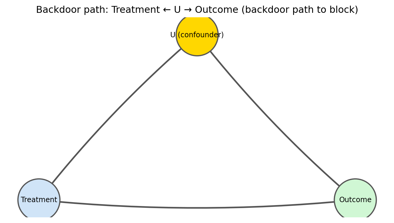
Figure 6.1: Backdoor paths in a simple DAG. The confounder U creates a spurious path between Treatment and Outcome.
6.5 Summary
Observing \(P(Y \mid X)\) and intervening \(P(Y \mid do(X))\) are different quantities; they coincide only when there are no confounders.
The do-operator corresponds to removing incoming edges to the target node — the “mutilated graph.”
The backdoor criterion identifies a set of observed variables that, if adjusted for, removes confounding and yields the causal effect.
The front-door criterion allows causal identification even when confounders are unobserved, using a mediating variable.
6.6 Further Reading
Pearl (2009) contains the full derivation of the do-calculus and its completeness. The three rules of the do-calculus are stated in Chapter 3; the backdoor and front-door criteria are in Chapter 3–4. Pearl and Mackenzie (2018) retells these results with historical narrative in Chapters 7–8.
Pearl, Judea. 2009. Causality: Models, Reasoning, and Inference. 2nd ed. Cambridge University Press.
Pearl, Judea, and Dana Mackenzie. 2018. The Book of Why: The New Science of Cause and Effect. Basic Books.
Source Code
---title: "Interventions and the Do-Calculus"---::: {.callout-note icon=false}## Learning Objectives- Distinguish between observing a variable and intervening on it- Understand the do-operator and what it means to "cut" a DAG- Apply the backdoor criterion to identify confounders and adjust for them- Work through a front-door adjustment when backdoor adjustment is impossible:::## Seeing vs. DoingThere is a profound difference between learning that someone takes aspirin frequently and *making* someone take aspirin. The first is an observation. The second is an intervention.When we observe that heavy aspirin users have lower rates of heart disease, we cannot immediately conclude that aspirin prevents heart disease. Perhaps people who take aspirin regularly are also more health-conscious in other ways — they exercise, avoid smoking, see their doctors more often. The observation conflates the effect of aspirin with the effect of health-consciousness.When we intervene — assigning aspirin randomly to participants in a clinical trial — we sever the link between aspirin use and whatever background factors made someone likely to take aspirin in the first place. We have, in effect, *cut* the incoming arrows to the aspirin node in the causal graph.Pearl's notation captures this precisely. The expression $P(Y \mid X = x)$ asks: among people we *observe* to have $X = x$, what is the distribution of $Y$? The expression $P(Y \mid do(X = x))$ asks: if we *set* $X = x$ by intervention, what would the distribution of $Y$ be?These two quantities can differ dramatically.## Interventional Distributions and the Mutilated GraphMathematically, computing $P(Y \mid do(X = x))$ corresponds to:1. Remove all incoming arrows to $X$ from the DAG (the "mutilated graph").2. Fix $X = x$.3. Compute the probability of $Y$ in this modified graph.The mutilated graph represents a world in which the variable $X$ is under external control — no longer influenced by its natural causes.## The Backdoor CriterionFor most practical applications, we want to estimate causal effects from observational data — without a randomized experiment. The backdoor criterion tells us when, and how, this is possible.A set of variables $Z$ satisfies the **backdoor criterion** relative to an ordered pair $(X, Y)$ if:1. No node in $Z$ is a descendant of $X$.2. $Z$ blocks every "backdoor path" from $X$ to $Y$ — every path that begins with an arrow *into* $X$.If such a $Z$ exists, the causal effect of $X$ on $Y$ can be estimated by adjusting for $Z$:$$P(Y \mid do(X)) = \sum_z P(Y \mid X, Z = z) \cdot P(Z = z)$$ {#eq-backdoor}This is the adjustment formula. In a regression context, it corresponds to including the confounders $Z$ as covariates.## The Front-Door CriterionSometimes no valid adjustment set exists — the confounders are unobserved. The front-door criterion offers an alternative route in certain graph structures.If there is a mediator $M$ between $X$ and $Y$ such that: (1) all paths from $X$ to $Y$ go through $M$, (2) there are no unblocked backdoor paths from $X$ to $M$, and (3) all backdoor paths from $M$ to $Y$ are blocked by $X$ — then the causal effect can be estimated even without observing the confounders:$$P(Y \mid do(X)) = \sum_m P(M = m \mid X) \sum_x P(Y \mid X = x, M = m) P(X = x)$$ {#eq-frontdoor}The front-door adjustment was Pearl's demonstration that causal inference is sometimes possible even when all the confounders are hidden.```{python}#| label: fig-backdoor-dag#| fig-cap: "Backdoor paths in a simple DAG. The confounder U creates a spurious path between Treatment and Outcome."import networkx as nximport matplotlib.pyplot as pltG = nx.DiGraph()nodes = ["U (confounder)", "Treatment", "Outcome"]edges = [ ("U (confounder)", "Treatment"), ("U (confounder)", "Outcome"), ("Treatment", "Outcome"),]G.add_nodes_from(nodes)G.add_edges_from(edges)pos = {"U (confounder)": (1, 2), "Treatment": (0, 0), "Outcome": (2, 0)}colors = {"U (confounder)": "#ffd700", "Treatment": "#d0e4f7", "Outcome": "#d0f7d4"}fig, ax = plt.subplots(figsize=(7, 4))nx.draw_networkx_nodes(G, pos, ax=ax, node_size=2800, node_color=[colors[n] for n in G.nodes()], edgecolors="#555", linewidths=1.5)nx.draw_networkx_labels(G, pos, ax=ax, font_size=9)nx.draw_networkx_edges(G, pos, ax=ax, arrows=True, arrowsize=25, edge_color="#555", width=2, connectionstyle="arc3,rad=0.05")ax.set_title("Backdoor path: Treatment ← U → Outcome (backdoor path to block)")ax.axis("off")plt.tight_layout()plt.show()```## Summary- Observing $P(Y \mid X)$ and intervening $P(Y \mid do(X))$ are different quantities; they coincide only when there are no confounders.- The do-operator corresponds to removing incoming edges to the target node — the "mutilated graph."- The backdoor criterion identifies a set of observed variables that, if adjusted for, removes confounding and yields the causal effect.- The front-door criterion allows causal identification even when confounders are unobserved, using a mediating variable.## Further Reading@pearl2009causality contains the full derivation of the do-calculus and its completeness. The three rules of the do-calculus are stated in Chapter 3; the backdoor and front-door criteria are in Chapter 3–4. @pearl2018book retells these results with historical narrative in Chapters 7–8.