Understand what a Directed Acyclic Graph (DAG) represents in causal modeling
Apply the d-separation criterion to determine conditional independence
Describe Pearl’s Ladder of Causation and the three rungs
Build and visualize a simple DAG using Python
5.1 Drawing the Story
A Directed Acyclic Graph is a picture with a purpose. Each node represents a variable. Each directed edge represents a direct causal relationship: an arrow from \(X\) to \(Y\) means \(X\) is one of the direct causes of \(Y\). “Acyclic” means the graph has no loops — you cannot follow arrows from any node and return to where you started. This rules out feedback cycles, which require a different formalism entirely.
The graph encodes qualitative causal structure: which things affect which other things, independent of the precise functional form or the strength of the effect. This separation of structure from magnitude is one of the most powerful features of the causal framework. It lets you reason about what you can and cannot learn from data before you even look at the numbers.
5.2 d-Separation and Conditional Independence
Not every pair of variables in a DAG is associated. Whether two nodes \(X\) and \(Y\) are statistically dependent — or independent, or conditionally independent given some third variable \(Z\) — is determined by the paths connecting them and the role of \(Z\) in those paths.
Judea Pearl’s d-separation criterion provides the exact rules. Three patterns matter:
Chain:\(X \to Z \to Y\) — \(Z\) mediates the relationship between \(X\) and \(Y\). Conditioning on \(Z\) blocks the path: \(X \perp Y \mid Z\).
Fork:\(X \leftarrow Z \to Y\) — \(Z\) is a common cause. The association between \(X\) and \(Y\) is due to \(Z\). Conditioning on \(Z\) blocks the path.
Collider:\(X \to Z \leftarrow Y\) — \(Z\) is caused by both \(X\) and \(Y\). Without conditioning, the path is blocked: \(X \perp Y\). But if you condition on \(Z\), the path opens: \(X \not\perp Y \mid Z\).
This last case is the collider phenomenon from Chapter 4, now stated precisely.
5.3 The Ladder of Causation
Pearl describes three levels of causal reasoning, which he calls the Ladder of Causation:
Rung 1 — Association. What do I see? Statistical patterns, correlations, conditional expectations. This is the domain of observational data and classical machine learning. A camera captures this rung.
Rung 2 — Intervention. What happens if I do something? The question is no longer about observations but about actions — about changing the world and observing the consequences. A thermostat operates on this rung. This is the domain of randomized experiments and the do-calculus (Chapter 6).
Rung 3 — Counterfactuals. What would have happened if things had been different? This rung asks about worlds that did not occur. It is the domain of law (was this the proximate cause of the accident?), medicine (would this patient have survived without the treatment?), and moral philosophy. It requires the full machinery of structural causal models.
Most statistical methods operate exclusively on Rung 1. They are, in this sense, blind to the questions on Rungs 2 and 3 — not because they lack data, but because the questions themselves live at a higher level of the ladder.
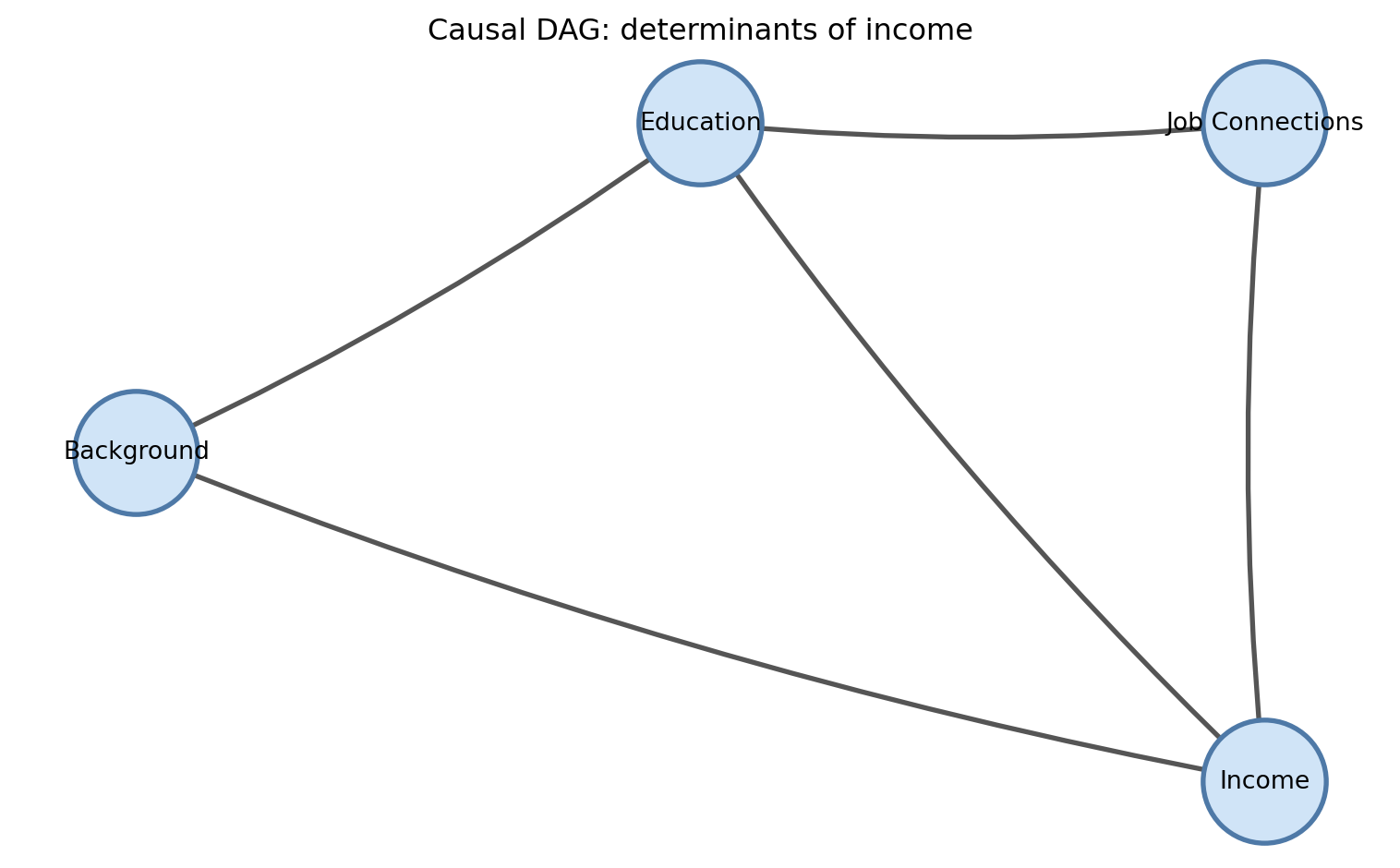
Figure 5.1: A simple causal DAG: education and background both influence income; background also influences education.
5.4 Summary
A DAG is a qualitative description of causal structure: nodes are variables, directed edges are direct causal relationships.
d-separation determines which pairs of variables are conditionally independent, given a set of observed variables.
The three fundamental path patterns — chain, fork, collider — each have different independence implications.
The Ladder of Causation distinguishes association (what is), intervention (what would be if I acted), and counterfactuals (what would have been if things had been different).
5.5 Further Reading
Pearl (2009) is the definitive technical reference for DAGs and d-separation. For a shorter introduction, Chapter 3 of Pearl and Mackenzie (2018) covers the same ground for a general audience. The pgmpy library (used in later chapters) provides Python tools for constructing and querying Bayesian networks.
Pearl, Judea. 2009. Causality: Models, Reasoning, and Inference. 2nd ed. Cambridge University Press.
Pearl, Judea, and Dana Mackenzie. 2018. The Book of Why: The New Science of Cause and Effect. Basic Books.
Source Code
---title: "Structural Causal Models and DAGs"---::: {.callout-note icon=false}## Learning Objectives- Understand what a Directed Acyclic Graph (DAG) represents in causal modeling- Apply the d-separation criterion to determine conditional independence- Describe Pearl's Ladder of Causation and the three rungs- Build and visualize a simple DAG using Python:::## Drawing the StoryA Directed Acyclic Graph is a picture with a purpose. Each node represents a variable. Each directed edge represents a direct causal relationship: an arrow from $X$ to $Y$ means $X$ is one of the direct causes of $Y$. "Acyclic" means the graph has no loops — you cannot follow arrows from any node and return to where you started. This rules out feedback cycles, which require a different formalism entirely.The graph encodes *qualitative* causal structure: which things affect which other things, independent of the precise functional form or the strength of the effect. This separation of structure from magnitude is one of the most powerful features of the causal framework. It lets you reason about what you can and cannot learn from data before you even look at the numbers.## d-Separation and Conditional IndependenceNot every pair of variables in a DAG is associated. Whether two nodes $X$ and $Y$ are statistically dependent — or independent, or conditionally independent given some third variable $Z$ — is determined by the *paths* connecting them and the role of $Z$ in those paths.Judea Pearl's d-separation criterion provides the exact rules. Three patterns matter:**Chain:** $X \to Z \to Y$ — $Z$ mediates the relationship between $X$ and $Y$. Conditioning on $Z$ blocks the path: $X \perp Y \mid Z$.**Fork:** $X \leftarrow Z \to Y$ — $Z$ is a common cause. The association between $X$ and $Y$ is due to $Z$. Conditioning on $Z$ blocks the path.**Collider:** $X \to Z \leftarrow Y$ — $Z$ is caused by both $X$ and $Y$. Without conditioning, the path is blocked: $X \perp Y$. But if you condition on $Z$, the path opens: $X \not\perp Y \mid Z$.This last case is the collider phenomenon from Chapter 4, now stated precisely.## The Ladder of CausationPearl describes three levels of causal reasoning, which he calls the Ladder of Causation:**Rung 1 — Association.** What do I see? Statistical patterns, correlations, conditional expectations. This is the domain of observational data and classical machine learning. A camera captures this rung.**Rung 2 — Intervention.** What happens if I do something? The question is no longer about observations but about *actions* — about changing the world and observing the consequences. A thermostat operates on this rung. This is the domain of randomized experiments and the do-calculus (Chapter 6).**Rung 3 — Counterfactuals.** What would have happened if things had been different? This rung asks about worlds that did not occur. It is the domain of law (*was this the proximate cause of the accident?*), medicine (*would this patient have survived without the treatment?*), and moral philosophy. It requires the full machinery of structural causal models.Most statistical methods operate exclusively on Rung 1. They are, in this sense, blind to the questions on Rungs 2 and 3 — not because they lack data, but because the questions themselves live at a higher level of the ladder.```{python}#| label: fig-dag-example#| fig-cap: "A simple causal DAG: education and background both influence income; background also influences education."import networkx as nximport matplotlib.pyplot as pltimport matplotlib.patches as mpatchesG = nx.DiGraph()nodes = ["Background", "Education", "Income", "Job Connections"]edges = [ ("Background", "Education"), ("Background", "Income"), ("Education", "Income"), ("Education", "Job Connections"), ("Job Connections", "Income"),]G.add_nodes_from(nodes)G.add_edges_from(edges)pos = {"Background": (0, 1),"Education": (1, 2),"Job Connections": (2, 2),"Income": (2, 0),}fig, ax = plt.subplots(figsize=(8, 5))nx.draw_networkx_nodes(G, pos, ax=ax, node_size=2500, node_color="#d0e4f7", edgecolors="#4e79a7", linewidths=2)nx.draw_networkx_labels(G, pos, ax=ax, font_size=10)nx.draw_networkx_edges(G, pos, ax=ax, arrows=True, arrowsize=25, edge_color="#555", width=2, connectionstyle="arc3,rad=0.05")ax.set_title("Causal DAG: determinants of income")ax.axis("off")plt.tight_layout()plt.show()```## Summary- A DAG is a qualitative description of causal structure: nodes are variables, directed edges are direct causal relationships.- d-separation determines which pairs of variables are conditionally independent, given a set of observed variables.- The three fundamental path patterns — chain, fork, collider — each have different independence implications.- The Ladder of Causation distinguishes association (what is), intervention (what would be if I acted), and counterfactuals (what would have been if things had been different).## Further Reading@pearl2009causality is the definitive technical reference for DAGs and d-separation. For a shorter introduction, Chapter 3 of @pearl2018book covers the same ground for a general audience. The `pgmpy` library (used in later chapters) provides Python tools for constructing and querying Bayesian networks.